Accurate approximation of collision integrals using Neufeld’s empirical equations
Authors: Housam Binous and Ahmed Bellagi
Accurate approximation of collision integrals using Neufeld’s empirical equations
Authors: Housam Binous and Ahmed Bellagi
Authors: Housam Binous and Ahmed Bellagi
Ω
D
Ω
D
Ω
k
Ω
μ
κT/
ϵ
AB
-16
10
ϵ
AB
Collision integral for mass diffusivity or
Ω
D
In[]:=
Clear[A,B,C1,D1,E1,F,G,H,R,S,W,P]
In[]:=
OMEGA11=A/TS^B+C1/Exp[D1TS]+E1/Exp[FTS]+G/Exp[HTS]
Out[]=
C1+E1+G+A
-D1TS
-FTS
-HTS
-B
TS
In[]:=
A=1.06036;B=0.15610;C1=0.19300;D1=0.47635;E1=1.03587;F=1.52996;G=1.76474;H=3.89411;
In[]:=
data={{0.3,2.662},{0.35,2.476},{0.4,2.318},{0.45,2.184},{0.5,2.066},{0.55,1.966},{0.6,1.877},{0.65,1.798},{0.7,1.729},{0.75,1.667},{0.8,1.612},{0.85,1.562},{0.9,1.517},{0.95,1.476},{1.,1.439},{1.05,1.406},{1.1,1.375},{1.15,1.346},{1.2,1.32},{1.25,1.296},{1.3,1.273},{1.35,1.253},{1.4,1.233},{1.45,1.215},{1.5,1.198},{1.55,1.182},{1.6,1.167},{1.65,1.153},{1.8,1.116},{1.85,1.105},{1.9,1.094},{1.95,1.084},{2.,1.075},{2.1,1.057},{2.2,1.041},{2.3,1.026},{2.4,1.012},{2.5,0.9996},{2.6,0.9878},{2.7,0.977},{2.8,0.9672},{2.9,0.9576},{3.,0.949},{3.1,0.9406},{3.2,0.9328},{3.3,0.9256},{3.4,0.9186},{3.5,0.912},{3.6,0.9058},{3.7,0.8998},{3.8,0.8942},{3.9,0.8888},{4.,0.8836},{4.1,0.8788},{4.2,0.874},{4.3,0.8694},{4.4,0.8652},{4.5,0.861},{4.6,0.8568},{4.7,0.853},{4.8,0.8492},{4.9,0.8456},{5.,0.8422},{6.,0.8124},{7.,0.7896},{8.,0.7712},{10.,0.7424},{20.,0.664},{30.,0.6232},{40.,0.596},{50.,0.5756},{60.,0.5596},{70.,0.5464},{80.,0.5352},{90.,0.5256}};(*datafromappendixKofRef.1*)
In[]:=
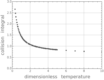
p1=ListPlot[data,Frame->True,GridLines->Automatic,AspectRatio->0.75,ImageSize->Medium,FrameLabel->{Style["dimensionless temperature",16],Style["collision integral",16]},PlotStyle->Darker@Gray,PlotRange->{{0,10},{0,3}}]
Out[]=
In[]:=
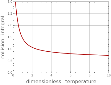
p2=Plot[OMEGA11,{TS,0.05,15},Frame->True,GridLines->Automatic,AspectRatio->0.75,ImageSize->Medium,FrameLabel->{Style["dimensionless temperature",16],Style["collision integral",16]},PlotStyle->Darker@Red,PlotRange->{{0,10},{0,3}}]
Out[]=
In[]:=
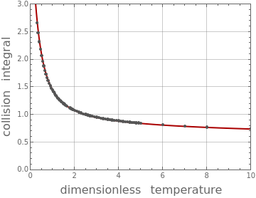
Show[p2,p1]
Out[]=
Collision integral for viscosity and thermal conductivity or and
Ω
μ
Ω
k
In[]:=
Clear[A,B,C1,D1,E1,F,G,H,R,S,W,P]
In[]:=
OMEGA22=A/TS^B+C1/Exp[D1TS]+E1/Exp[FTS]+RTS^BSin[STS^W-P]
Out[]=
C1+E1+A-RSin[P-S]
-D1TS
-FTS
-B
TS
B
TS
W
TS
In[]:=
A=1.16145;B=0.14874;C1=0.52487;D1=0.77320;E1=2.16178;F=2.43787;W=-0.76830;P=7.27371;R=-6.43510^-4;S=18.0323;
In[]:=
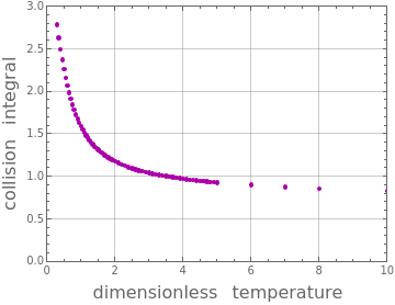
data={{0.3,2.785},{0.35,2.628},{0.4,2.492},{0.45,2.368},{0.5,2.257},{0.55,2.156},{0.6,2.065},{0.65,1.982},{0.7,1.908},{0.75,1.841},{0.8,1.78},{0.85,1.725},{0.9,1.675},{0.95,1.629},{1.,1.587},{1.05,1.549},{1.1,1.514},{1.15,1.482},{1.2,1.452},{1.25,1.424},{1.3,1.399},{1.35,1.375},{1.4,1.353},{1.45,1.333},{1.5,1.314},{1.55,1.296},{1.6,1.279},{1.65,1.264},{1.7,1.248},{1.8,1.221},{1.85,1.209},{1.9,1.197},{1.95,1.186},{2.,1.175},{2.1,1.156},{2.2,1.138},{2.3,1.122},{2.4,1.107},{2.5,1.093},{2.6,1.081},{2.7,1.069},{2.8,1.058},{2.9,1.048},{3.,1.039},{3.1,1.03},{3.2,1.022},{3.3,1.014},{3.4,1.007},{3.5,0.9999},{3.6,0.9932},{3.7,0.987},{3.8,0.9811},{3.9,0.9755},{4.,0.97},{4.1,0.9649},{4.2,0.96},{4.3,0.9553},{4.4,0.9507},{4.5,0.9464},{4.6,0.9422},{4.7,0.9382},{4.8,0.9343},{4.9,0.9305},{5.,0.9269},{6.,0.8963},{7.,0.8727},{8.,0.8538},{10.,0.8242},{20.,0.7432},{30.,0.7005},{40.,0.6718},{50.,0.6504},{60.,0.6335},{70.,0.6194},{80.,0.6076},{90.,0.5973}};(*datafromappendixKofRef.1*)
In[]:=
p1b=ListPlot[data,Frame->True,GridLines->Automatic,AspectRatio->0.75,ImageSize->Medium,FrameLabel->{Style["dimensionless temperature",16],Style["collision integral",16]},PlotStyle->Darker@Magenta,PlotRange->{{0,10},{0,3}}]
Out[]=
In[]:=
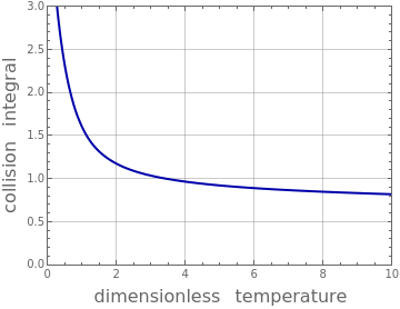
p2b=Plot[OMEGA22,{TS,0.05,15},Frame->True,GridLines->Automatic,AspectRatio->0.75,ImageSize->Medium,FrameLabel->{Style["dimensionless temperature",16],Style["collision integral",16]},PlotStyle->Darker@Blue,PlotRange->{{0,10},{0,3}}]
Out[]=