Analyzing the spread of SARS-CoV-2 variants in California
by Daniel Lichtblau
by Daniel Lichtblau
Introduction
Introduction
I was informed yesterday of an article in the LA Times about the rise in California COVID-19 cases due to what is of late called the “California strain”.
This strain is comprised of the B.1.429 and B.1.427 variants. Also mentioned in the article is the variant that originally arose in England, B.1.1.7. Both are in California and both are believed to be more contagious than the original and most subsequent forms of SARS-CoV-2. As it happens, I have been making some effort to track these two variants in California for the past three weeks or so. I had initially thought B.1.1.7 might take over as the dominant strain, as has apparently happened in several parts of Europe. What I have been seeing, however, does not support this. It seems that only the California variant is gathering steam.
The data I use comes from GISAID. One has to register to use this site, and it is subject to certain requirements in terms of attribution. To this end, I include all annotations for the sequences utilized below, in a supplementary section at the end of this note. First I will show how a download appears in my browser.
Out[]=
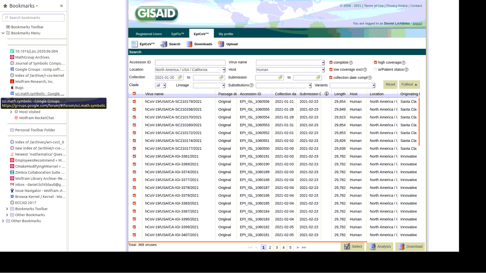
As can be seen in the screenshot, I checked boxes to get only sequences that are nearly or entirely complete. The ones above are recent California sequences, specifically, those from specimens collected on or after January 20. I also grabbed all USA sequences of the B.1.1.7 variant that were collected between January 1 and January 19. I stop at that date in order to be certain not to have overlaps with the recent California sequences. My third set is comprised of California sequences that are classified as the B.1.429 variant and were collected between January 1 and January 14. I chose January 14 as the stop date again to be sure to avoid overlaps in the three groups, and also to keep the sizes of the three sets comparable.
The method I use for classification is described in a pair of prior Wolfram Community posts. The first is from February 7, 2020, (mis-)named Genome analysis and the SARS-nCoV-2 (the “n” before “CoV” should not be present). Here I only tried to classify various Coronaviruses, and made no attempt to get to the level of variants. The second Community post, From sequenced SARS-CoV-2 genomes to a phylogenetic tree, goes into more detail on the method used to create a phylogenetic tree from a set of genome sequences. In both posts there is some explanation also of a visualization method based on Multidimensional Scaling (MDS). I use that method below to place genome sequences as points in three dimensions. A color scheme will then indicate proximities between sequences.
Loading and processing the genome sequences
Loading and processing the genome sequences
First I load GISAID recent California sequences, specifically, those collected on or after January 20 and placed in GISAID by February 25. As will be seen from the code, I have stored these in the Downloads subdirectory of my home directory.
In[]:=
dropTrailingA[seq_]:=StringReplace[seq,StartOfString~~Shortest[a__]~~("A"..)~~EndOfStringa];
filenameCA="GISAID_CA_JAN20.fasta";gisCAJAN20PlusSeqs=Map[dropTrailingA,Import[FileNameJoin[{$HomeDirectory,"Downloads",filenameCA}],"FASTA"]];gisCAJAN20PlusIDStrings=Select[ss=StringSplit[Import[FileNameJoin[{$HomeDirectory,"Downloads",filenameCA}],"Text"],"\n"],StringMatchQ[#,">hCoV"~~___]&];Map[Length,{gisCAJAN20PlusSeqs,gisCAJAN20PlusIDStrings}]
Out[]=
{368,368}
The code below simply colors the sequences by collection date. Earlier ones are green, with a change toward purple for the most recent sequences.
{gisCAJAN20PlusNames0,gisCAJAN20PlusAscensions,gisCAJAN20PlusDates0}=Transpose[StringSplit[gisCAJAN20PlusIDStrings,"|"]];gisCAJAN20PlusDates=ToExpression[Map[StringSplit[#,"-"]&,gisCAJAN20PlusDates0]];{gisCAJAN20PlusCountries,gisCAJAN20PlusNames,gisCAJAN20PlusYears}=Transpose@Map[StringSplit[#,"/"]&,gisCAJAN20PlusNames0][[All,2;;]];ngisCAJAN20PlusDates=Map[(#[[1]]-2020)*365+(#[[2]])*30.4+#[[3]]-410&,gisCAJAN20PlusDates];ndatesCAJAN20=.4*Rescale[ngisCAJAN20PlusDates]+.02;colorbydateCAJAN20=Thread[Style[gisCAJAN20PlusDates,Map[Darker[Hue[#]]&,ngisCAJAN20PlusDates]]];Short[Sort@colorbydateCAJAN20,3]
Out[]//Short=
{{2021,1,20},{2021,1,20},{2021,1,20},{2021,1,20},{2021,1,20},{2021,1,20},{2021,1,20},{2021,1,20},{2021,1,20},{2021,1,20},{2021,1,20},{2021,1,20},{2021,1,20},342,{2021,2,9},{2021,2,9},{2021,2,9},{2021,2,9},{2021,2,9},{2021,2,9},{2021,2,10},{2021,2,10},{2021,2,11},{2021,2,12},{2021,2,12},{2021,2,12},{2021,2,12}}
I convert sequences to fixed size images using the “Frequency Chaos Game Representation” (FCGR). For this I use a function from the Wolfram Function Repository.
In[]:=
gisCAJAN20Plusfcgrs=Map[ResourceFunction["FCGRImage"],gisCAJAN20PlusSeqs];gisCAJAN20Plusftts=Map[Flatten[FourierDCT[#-Mean[Flatten[#]],4][[1;;30,1;;30]]]&,Map[ImageData,gisCAJAN20Plusfcgrs]];
I now similarly load and process GISAID USA B.1.1.7 sequences collected from 2021-01-01 through 2020-01-19
In[]:=
filenameUSAB117="GISAID_USA_JAN01_JAN19_B_1_1_7.fasta";gisUSAB117Seqs=Map[dropTrailingA,Import[FileNameJoin[{$HomeDirectory,"Downloads",filenameUSAB117}],"FASTA"]];gisUSAB117IDStrings=Select[ss=StringSplit[Import[FileNameJoin[{$HomeDirectory,"Downloads",filenameUSAB117}],"Text"],"\n"],StringMatchQ[#,">hCoV"~~___]&];Map[Length,{gisUSAB117Seqs,gisUSAB117IDStrings}]
Out[]=
{360,360}
These B.1.1.7 sequences will all be colored gray for purposes of visualization below.
In[]:=
colorsUSAB117=ConstantArray[Gray,Length[gisUSAB117Seqs]];
In[]:=
gisUSAB117fcgrs=Map[ResourceFunction["FCGRImage"],gisUSAB117Seqs];gisUSAB117ftts=Map[Flatten[FourierDCT[#-Mean[Flatten[#]],4][[1;;30,1;;30]]]&,Map[ImageData,gisUSAB117fcgrs]];
And we load and process GISAID California B.1.429 sequences collected from 2021-01-01 through 2020-01-14
In[]:=
filenameCAB1429="GISAID_CA_JAN01_JAN14_B_1_429.fasta";gisCAB1429Seqs=Map[dropTrailingA,Import[FileNameJoin[{$HomeDirectory,"Downloads",filenameCAB1429}],"FASTA"]];gisCAB1429IDStrings=Select[ss=StringSplit[Import[FileNameJoin[{$HomeDirectory,"Downloads",filenameCAB1429}],"Text"],"\n"],StringMatchQ[#,">hCoV"~~___]&];Map[Length,{gisCAB1429Seqs,gisCAB1429IDStrings}]
Out[]=
{423,423}
The B.1.429 sequences will all be colored blue.
In[]:=
colorsCAB1429=ConstantArray[Blue,Length[gisCAB1429Seqs]];
In[]:=
gisCAB1429fcgrs=Map[ResourceFunction["FCGRImage"],gisCAB1429Seqs];gisCAB1429ftts=Map[Flatten[FourierDCT[#-Mean[Flatten[#]],4][[1;;30,1;;30]]]&,Map[ImageData,gisCAB1429fcgrs]];
Multidimensional Scaling 3D plot
Multidimensional Scaling 3D plot
Now that we have preprocessed our sequences, we can reduce dimension further, to vectors of length 40. This uses a standard method involving the Singular Values Decomposition (SVD).
In[]:=
FTTsToVectors[ivecs_,keep_]:=Module[{uu,ww,vv,udotw,norms},{uu,ww,vv}=SingularValueDecomposition[ivecs,Min[keep,Length[ivecs]]];udotw=uu[[All,2;;]].ww[[2;;,2;;]];norms=Map[Sqrt[#.#]&,udotw];udotw=udotw/norms;udotw=Join[udotw,Transpose[{Log[norms]}],2];udotw]
smallervecsCAJAN20Plus=FTTsToVectors[Join[gisCAJAN20Plusftts,gisUSAB117ftts,gisCAB1429ftts],40];colorsCAPlus=Join[colorbydateCAJAN20[[All,2]],colorsUSAB117,colorsCAB1429];
In[]:=
skip=38;pl=PointLegend[Map[Darker[Hue[#]]&,Sort[ngisCAJAN20PlusDates][[1;;-1;;skip]]],Map[StringReplace[ToString[#],{"{""(","}"")"}]&,colorbydateCAJAN20[[Ordering[ngisCAJAN20PlusDates]]][[1;;-1;;skip]][[All,1,2;;]]],LegendLabel"color/(month/day)"];
In[]:=
styledMDSCAJAN20Plus3=Apply[Style,Thread[{ResourceFunction["MultidimensionalScaling"][smallervecsCAJAN20Plus,3],colorsCAPlus}],{1}];ListPointPlot3D[styledMDSCAJAN20Plus3,PlotRangeAll,PlotLegendspl]
Out[]=


One will see that the gray region has but few of the recent California sequences in its midst. The blue region, by contrast, contains roughly a third of the recent ones, and the proportion for the most recent (seen as purple dots) might be even higher. I will comment more about this picture, but first I will show how a phylogenetic tree gives confirmatory information.
A phylogenetic tree
A phylogenetic tree
In order to aid readability we decimate each set by a factor of four. The recent California SARS-CoV-2 genome sequences will be indicated by their date of collection, while the B.1.1.7 and B.1.429 variants will again be indicated by gray and blue markers respectively.
Again we see around a third of the recent sequences appearing in the midst of the B.1.429 variant, while very few are among the B.1.1.7 group. Of the most recent (purple), arond half appear within the B.1.429 subtree.
Remarks
Remarks
Both illustrations, the MDS plot and the phylogenetic tree, indicate that the B.1.1.7 variant is not at all close to becoming a dominant strain in California at this time. They also show that the B.1.429 variant might well be headed in that direction. Is this actually the case? There are several ways in which the illustrations might be misrepresenting the actual situation. I will discuss these and indicate why I believe they are not skewing the results in a large way.
1
.The underlying method of gauging proximity might not be very reliable. It is an alignment-free method and not likely to be as accurate as (much slower) direct edit-distance comparisons. I can say, however, that it stands up fairly well on many benchmark tests, some at the level of virus variants e.g. classification of HPV and the HxNy influenza viruses.
2
.The genome classifications in GISAID might be incorrect. This strikes me as unlikely. Certainly the B.1.1.7 sequences behave as one would expect, clumping together in both plots. The B.1.429 sequences seem to spread more (in the phylogenetic tree plot, this can be seen as longer branches emanating from their subtree). This could simply indicate that this variant has a greater tendency to mutate, or for other reasons is subject to greater variation. And there is another piece of information suggesting that we do not miss proximities to B.1.1.7 due to our methodology: a similar study, using sequences from Florida, does show a more noticeable increase there in prevalence of the B.1.1.7 variant. (It also shows that B.1.429 is in Florida, but that’s another matter.)
3
.Lack of sufficient data. This certainly is a possibility, especially given that SARS-CoV-2 sequencing is done far less in the US than in the UK. Nonetheless, each of the three groupings has a few hundred sequences, and this is a comparable amount to what I have seen in several similar studies.
4
.Geographic imbalances in where the California sequences are collected. It is possible, say, that the B.1.1.7 variant is gaining in a region that is contributing relatively less, per population, to the GISAID site. A spot check indicates that sequences are being provided by laboratories located both in southern and northern parts of California. This does not prove there is no imbalance, but at least suggests that such an imbalance, if it exists, is not terribly large. Moreover, I see consistent information when I replace the recent California sequences from GISAID with ones from GenBank.
5
.An MDS plot can show false proximities when the dimension reduction is larger than is warranted by the data. This is, in my experience, a problem that can arise in practice. But it has not, to date, been an issue (as best I can tell) in cases where the genome sequences utilized are close to complete. This is why I checked boxes on the GISAID site in a way that would exclude sequences of less than high quality. Also, when false proximity in an MDS plot is a problem, this is usually apparent in the phylogenetic tree; the sequences will appear better separated therein. For the data under scrutiny in this note, we see a comparable number of recent California sequences appearing within the B.1.429 grouping in both plots, and in the phylogenetic tree most branches separating recent sequences from known B.1.429 sequences are not terribly long.
6
.We might just be in the very early stages of B.1.1.7 presence in California. If so, this could account for very low percentage seen for that group. But B.1.1.7 was reported in California as far back as December 20, even earlier than first reports from Florida. At a doubling time of approximately 9 days (based on its approximated greater degree of infectiousness), we should see more of it in California at this time, were it really taking hold there.
Supplementary data
Supplementary data
GISAID sequence acknowledgements
GISAID sequence acknowledgements
Please click the button to expand the following