ABSTRACT (original article): The thermal degradation of anthocyanins in a variety of media and over a large temperature range is known to follow first-order kinetics, and the temperature-dependence of the exponential rate constant a two-parameter model. These parameters can be estimated from the initial and final concentrations of only two isothermal or non-isothermal heat treatments by numerically solving a pair of simultaneous equations of which they are the two unknowns. Once calculated they can be used to reconstruct the entire degradation curves and predict those of other heat treatments in a pertinent temperature range. Commercial mathematical software can do the calculations, as demonstrated with computer simulations and published data on the isothermal and non-isothermal degradation of anthocyanins. The endpoints method’s predictions were confirmed by comparison to the reported experimentally determined final concentrations. Where applicable, the method will eliminate the need to record sets of whole isothermal degradation curves in studies of the kinetics of anthocyanins’ degradation. Copyright © 2015 Elsevier Ltd. All rights reserved.
CITATION (original article): Peleg, M., Kim, A. D., & Normand, M. D. (2015). Predicting anthocyanins’ isothermal and non-isothermal degradation with the endpoints method. In Food Chemistry (Vol. 187, pp. 537–544). Elsevier BV. https://doi.org/10.1016/j.foodchem.2015.04.091
CITATION (original article): Peleg, M., Kim, A. D., & Normand, M. D. (2015). Predicting anthocyanins’ isothermal and non-isothermal degradation with the endpoints method. In Food Chemistry (Vol. 187, pp. 537–544). Elsevier BV. https://doi.org/10.1016/j.foodchem.2015.04.091
Introduction
Introduction
Theoretically, when a degradation reaction follows a known fixed-order kinetics, n, and the rate constant’s temperature-dependence follows a two-parameter model, then these parameters can be determined from two concentration ratios after exposure to two different temperature histories. This is done by numerically solving two simultaneous rate equations. Such a solution, however, may require fairly accurate initial guesses that are difficult to assign intuitively. Nevertheless, they can be estimated by manually matching the two experimental points with their corresponding degradation curves using Mathematica’s Manipulate function. Once found, they can be used either as initial guesses or as parameters themselves. In this program the degradation reaction rate’s temperature-dependence is described by the exponential model )] where T is the temperature, is the rate constant at a reference temperature, , and c is a constant. This program allows one to estimate and c by moving slider controls on the screen. The user enters the two digitized temperature profile data sets either by reading the data from a file or pasting them from another Mathematica notebook. Also entered using sliders are: the two final concentration ratios, the times at which they were determined and the reference temperature, . It is assumed that the reaction follows first-order kinetics or approximately first-order kinetics, in which case the deviation from n=1 can also be entered with a slider. The parameters’ settings in this program are for storage temperatures (Version A), and heat processing temperatures (Version B).
k(T)=k()*Exp[c*(T-
T
ref
T
ref
k()
T
ref
T
ref
k()
T
ref
T
ref
Notice that not all allowed entries for concentration ratios and times must result in a match. If there is no match one should suspect that either the model’s underlying assumptions are invalid and/or there is a substantial error or errors in the experimental data.
Version A - Storage
Version A - Storage
Import the first set of experimentally determined {time, temperature} data from a tab-separated-values (.TSV) ASCII text file into a matrix called tempData1A. Below we have pasted the data into this notebook so that no external file needs to be imported. If you want to import your own data from a file called “tempData1A.TSV” (located in your home folder), uncomment the cell below and comment out the cell after that which contains the assignment of the data to the tempData1A matrix.
(*tempData1A=Import["tempData1A.TSV"]*)
tempData1A={{0,25.`},{3.`,25.7`},{6.`,21.7`},{9.`,19.9`},{12.`,21.8`},{15.`,19.8`},{18.`,15.8`},{21.`,16.7`},{24.`,17.3`},{27.`,13.3`},{30.`,11.5`},{33.`,13.9`},{36.`,14.9`},{39.`,14.`},{42.`,12.3`},{45.`,11.5`},{48.`,12.4`},{51.`,14.9`},{54.`,17.3`},{57.`,18.2`},{60.`,17.3`},{63.`,15.6`},{66.`,14.8`},{69.`,15.8`},{72.`,18.3`},{75.`,20.7`},{78.`,21.6`},{81.`,20.6`},{84.`,19.`},{87.`,18.2`},{90.`,19.2`},{93.`,21.7`},{96.`,24.1`},{99.`,24.9`},{102.`,24.`},{105.`,22.3`},{108.`,21.5`},{111.`,22.6`},{114.`,25.1`},{117.`,27.5`},{120.`,28.3`}};
Display the number of time-temperature data values in matrix tempData1A and assign it to nPts1.
nPts1=Length[tempData1A]
41
Display the minimum temperature value in tempData1A.
Min[tempData1A[[All,2]]]
11.5
Display the maximum temperature value in tempData1A.
Max[tempData1A[[All,2]]]
28.3
Import the second set of experimentally determined {time, temperature} data from a second tab-separated-values (.TSV) ASCII text file into a matrix called tempData2A. Below we have pasted the data into this notebook so that no external file needs to be imported. If you want to import your own data from a file called “tempData2A.TSV” (located in your home folder), uncomment the cell below and comment out the cell after that which contains the assignment of the data to the tempData2A matrix.
(*tempData2A=Import["tempData2A.TSV"]*)
tempData2A=tempData1A[[1;;nPts1-5]];Do[tempData2A[[i,2]]=tempData1A[[i,2]]-.2*tempData1A[[i,1]],{i,nPts1-5}];tempData2A
{{0,25.},{3.,25.1},{6.,20.5},{9.,18.1},{12.,19.4},{15.,16.8},{18.,12.2},{21.,12.5},{24.,12.5},{27.,7.9},{30.,5.5},{33.,7.3},{36.,7.7},{39.,6.2},{42.,3.9},{45.,2.5},{48.,2.8},{51.,4.7},{54.,6.5},{57.,6.8},{60.,5.3},{63.,3.},{66.,1.6},{69.,2.},{72.,3.9},{75.,5.7},{78.,6.},{81.,4.4},{84.,2.2},{87.,0.8},{90.,1.2},{93.,3.1},{96.,4.9},{99.,5.1},{102.,3.6},{105.,1.3}}
Display the number of time-temperature data values in matrix tempData2A and assign it to nPts2.
nPts2=Length[tempData2A]
36
Display the minimum temperature value in tempData2A.
Min[tempData2A[[All,2]]]
0.8
Display the maximum temperature value in tempData2A.
Max[tempData2A[[All,2]]]
25.1
Assign tAxisMax1 and tMax1 to be the maximum time value found in matrix tempData1A.
tAxisMax1=Max[tempData1A[[All,1]]];tMax1=tAxisMax1
120.
Assign tAxisMax2 and tMax2 to be the maximum time value found in matrix tempData2A.
tAxisMax2=Max[tempData2A[[All,1]]];tMax2=tAxisMax2
105.
Assign TAxisMax1 and TMax1 to be the maximum Temperature value found in matrix tempData1A.
TAxisMax1=Max[tempData1A[[All,2]]];TMax1=TAxisMax1
28.3
TAxisMax1=40.
40.
Assign TAxisMax2 and TMax2 to be the maximum Temperature value found in matrix tempData2A.
TAxisMax2=Max[tempData2A[[All,2]]];TMax2=TAxisMax2
25.1
TAxisMax2=40.
40.
Assign T1 to be an interpolating function defined from the tempData1A points.
T1=Interpolation[tempData1A]
InterpolatingFunction[{{0.,120.}},<>]
Assign T2 to be an interpolating function defined from the tempData2A points.
T2=Interpolation[tempData2A]
InterpolatingFunction[{{0.,105.}},<>]
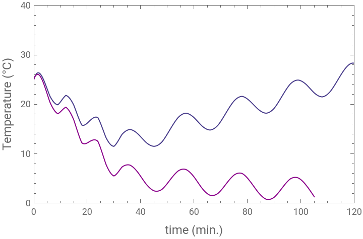
Plot the two interpolating functions T1[t] and T2[t] together from time 0 to Max[tAxisMax1,tAxisMax2].
temp1Plot=Plot[T1[t],{t,0,tMax1},PlotRange{{0,tAxisMax1},{0,TAxisMax1}},PlotStyle{AbsoluteThickness[1],ColorData["HTML","DarkSlateBlue"]},FrameTrue,FrameLabel{Style["time (min.)",12],Style["Temperature (°C)",12]}];
temp2Plot=Plot[T2[t],{t,0,tMax2},PlotRange{{0,tAxisMax2},{0,TAxisMax2}},PlotStyle{AbsoluteThickness[1],ColorData["HTML","DarkMagenta"]},FrameTrue,FrameLabel{Style["time (min.)",12],Style["Temperature (°C)",12]}];
T1T2Plot=Show[temp1Plot,temp2Plot,PlotRange{{0,Max[tAxisMax1,tAxisMax2]},{0,Max[TAxisMax1,TAxisMax2]}}]
Define ConcRatio(t), the degradation function obtained from the solution returned by NDSolve.
ConcRatio[tFinal_?NumericQ,kTref_?NumericQ,c_?NumericQ,n_?NumericQ,Tref_?NumericQ,T_]:=Module[{k,sfn,t,y},k[t_]:=kTref*Exp[c*(T[t]-Tref)];sfn[t_]=NDSolve[{y'[t]==-k[t]*y[t]^n,y[0]1.},y[t],{t,0.,tFinal},AccuracyGoal3][[1,1,2]];sfn[tFinal]]
The following Manipulate panel assists in selecting initial guesses for the kTref and c parameters of the ConcRatio(t) degradation function.
Manipulate[Module[{CExpPtsPlot,CPredPlot,CRatio1Plot,CRatio2Plot,kTrefcText,T1Plot,T2Plot,TParamText,T1T2Plot,TempMax,TempMin,tFinalEstConc3Text,tMax,yAxisMax},tMax=tAxisMax;yAxisMax=1.;tFinalEstConc3Text=Text[Style[Row[{""}],12]];kTrefcText=Text[Style[Row[{,"= ",Round[nAssumed,.01],Spacer[10],,"= ",Round[Treference,.01],Spacer[10],,"= ",Round[kTrefEst,.001],Spacer[10],,"= ",Round[cEst,.001]}],Blue,12]];T1Plot=Plot[T1[t],{t,0.,tMax1},PlotRange{{0.,tAxisMax},{0.,TAxisMax}},PlotStyle{AbsoluteThickness[1],ColorData["HTML","DarkSlateBlue"]},FrameTrue,FrameLabel{{Style["Temperature (°C)",12],""},{Style["time (arbitrary units)",12],Style["temperature profiles",12]}},ImagePadding{{45,10},{35,35}},ImageSize{360,222}];T2Plot=Plot[T2[t],{t,0.,tMax2},PlotRange{{0.,tAxisMax},{0.,TAxisMax}},PlotStyle{AbsoluteThickness[1],ColorData["HTML","DarkMagenta"]},FrameTrue,FrameLabel{{Style["Temperature (°C)",12],""},{Style["time (arbitrary units)",12],Style["temperature profiles",12]}},ImagePadding{{45,10},{35,35}},ImageSize{360,222}];CRatio1Plot=Plot[ConcRatio[t,kTrefEst,cEst,nAssumed,Treference,T1],{t,0.001,tMax1},PlotRange{{0.,tAxisMax},{-.05,yAxisMax}},PlotStyle{AbsoluteThickness[1],ColorData["HTML","DarkSlateBlue"]},FrameTrue,PlotLabel->kTrefcText,FrameLabel{{Style["concentration ratio(t)",12],""},{Style["time (arbitrary units)",12],Style["reconstructed degradation curves",12]}},ImagePadding{{45,10},{35,35}},ImageSize{360,222}];CRatio2Plot=Plot[ConcRatio[t,kTrefEst,cEst,nAssumed,Treference,T2],{t,0.001,tMax2},PlotRange{{0.,tAxisMax},{-.05,yAxisMax}},PlotStyle{AbsoluteThickness[1],ColorData["HTML","DarkMagenta"]},FrameTrue,PlotLabel->kTrefcText,FrameLabel{{Style["concentration ratio(t)",12],""},{Style["time (arbitrary units)",12],Style["reconstructed degradation curves",12]}},ImagePadding{{45,10},{35,35}},ImageSize{360,222}];CExpPtsPlot=ListPlot[{{{tFinal1,Cexper1}},{{tFinal2,Cexper2}}},PlotRange{{0.,tAxisMax},{-.05,yAxisMax}},PlotStyle{{AbsolutePointSize[6],ColorData["HTML","DarkSlateBlue"]},{AbsolutePointSize[6],ColorData["HTML","DarkMagenta"]}},FrameTrue,FrameLabel{{Style["concentration ratio(t)",12],""},{Style["time (arbitrary units)",12]}},ImagePadding{{45,10},{35,35}},ImageSize{360,222}];T1T2Plot=Show[T1Plot,T2Plot];Column[{tFinalEstConc3Text,T1T2Plot,Show[CRatio1Plot,CRatio2Plot,CExpPtsPlot]}]],Style["kinetic parameter estimation",Bold,9],{{tFinal1,tMax1,},10.,600.,Appearance"Labeled",ImageSizeSmall},{{Cexper1,.5,},.1,.95,Appearance"Labeled",ImageSizeSmall},"\n",{{tFinal2,tMax2,},10.,600.,Appearance"Labeled",ImageSizeSmall},{{Cexper2,.85,},.1,.95,Appearance"Labeled",ImageSizeSmall},Delimiter,Style["assumed kinetic order",Bold,9],{{nAssumed,1.,},.95,1.05,.01,Appearance"Labeled",ImageSizeSmall},Delimiter,Style["reference temperature",Bold,9],{{Treference,20.,},20.,80.,Appearance"Labeled",ImageSizeSmall},Delimiter,Style["estimated degradation's parameters",Bold,9],{{kTrefEst,.0055,},.0001,.2,Appearance"Labeled",ImageSizeSmall},{{cEst,.149,},.0001,.2,Appearance"Labeled",ImageSizeSmall},Delimiter,Style["time axis maximum",Bold,9],{{tAxisMax,140.,},10.,600.,Appearance"Labeled",ImageSizeSmall},Style["Temperature axis maximum",Bold,9],{{TAxisMax,40.,},10.,150.,Appearance"Labeled",ImageSizeSmall},ControlPlacementLeft,SaveDefinitionsTrue,AutorunSequencingAutomatic,TrackedSymbols{tFinal1,Cexper1,tFinal2,Cexper2,nAssumed,Treference,kTrefEst,cEst,tAxisMax,TAxisMax}]
Style["n",Italic]
as
Style["T",Italic]
ref
Style["k",Italic]
Trefest
Style["c",Italic]
est
Style["t",Italic]
final1
Style["C",Italic]
exper1
Style["t",Italic]
final2
Style["C",Italic]
exper2
Style["n",Italic]
assumed
Style["T",Italic]
ref
Style["k",Italic]
Trefest
Style["c",Italic]
est
Style["t",Italic]
max
Style["T",Italic]
max
Version B - Heat Processing
Version B - Heat Processing
Import the first set of experimentally determined {time, temperature} data from a tab-separated-values (.TSV) ASCII text file into a matrix called tempData1B. Below we have pasted the data into this notebook so that no external file needs to be imported. If you want to import your own data from a file called “tempData1.tsv” (located in your home folder), uncomment the cell below and comment out the cell after that which contains the assignment of the data to the tempData1B matrix.
Display the number of time-temperature data values in matrix tempData1B and assign it to nPts1.
Display the minimum temperature value in tempData1B.
Display the maximum temperature value in tempData1B.
Import the second set of experimentally determined {time, temperature} data from a second tab-separated-values (.TSV) ASCII text file into a matrix called tempData2B. Below we have pasted the data into this notebook so that no external file needs to be imported. If you want to import your own data from a file called “tempData2.TSV” (located in your home folder), uncomment the cell below and comment out the cell after that which contains the assignment of the data to the tempData2B matrix.
Display the number of time-temperature data values in matrix tempData2B and assign it to nPts2.
Display the minimum temperature value in tempData2B.
Display the maximum temperature value in tempData2B.
Assign tAxisMax1 and tMax1 to be the maximum time value found in matrix tempData1B.
Assign tAxisMax2 and tMax2 to be the maximum time value found in matrix tempData2B.
Assign TAxisMax1 and TMax1 to be the maximum Temperature value found in matrix tempData1B.
Assign TAxisMax2 and TMax2 to be the maximum Temperature value found in matrix tempData2B.
Assign T1 to be an interpolating function defined from the tempData1B points.
Assign T2 to be an interpolating function defined from the tempData2B points.
Plot the two interpolating functions T1[t] and T2[t] together from time 0 to Max[tAxisMax1,tAxisMax2].
Define ConcRatio(t), the degradation function obtained from the solution returned by NDSolve.
The following Manipulate panel assists in selecting initial guesses for the kTref and c parameters of the ConcRatio(t) degradation function.
Development Project
Development Project
Developed as part of a project on vitamin loss kinetics in space foods supported by NASA under project SA-14-042.
Related Articles
Related Articles
◼
[1] M. Peleg, M. D. Normand and A. D. Kim, “Estimating Nutrients’ Thermal Degradation Kinetic Parameters with the Endpoints Method,” Food Research International, 66, 2014 pp. 313-324.
◼
[2] M. Peleg, A. D. Kim and M. D. Normand, “Predicting anthocyanin’s isothermal and non-isothermal degradation with the endpoints method” Food Chemistry, 2015 (in press).
◼
[3] M. Peleg, M. D. Normand and M. G. Corradini, “The Arrhenius equation revisited,” Critical Reviews in Foods Science and Nutrition, 52, 2012 pp. 830-851.
CITE THIS NOTEBOOK
CITE THIS NOTEBOOK
Degradation parameters estimation from interpolated temperature data
by Micha Peleg and Mark D. Normand
Wolfram Community, STAFF PICKS, April 3, 2024
https://community.wolfram.com/groups/-/m/t/3152258
by Micha Peleg and Mark D. Normand
Wolfram Community, STAFF PICKS, April 3, 2024
https://community.wolfram.com/groups/-/m/t/3152258