ABSTRACT (original article): Water is crucial in a modern society, with potable water provided for households, coolant water for electrical power plants, and as a solvent for the pharmaceutical and biochemical industries. The dynamic range of water flow measurements has grown to meet the needs from these industrial sectors. At present, the lowest flow rate is 0.2 μg/s, while the highest flow rate is 20 kt/s for industrial applications.
This study explains the development of a water flow standard system at KRISS in South Korea. It has a flow range of 2.8 g/s (0.01 m³/h) to 0.56 t/s (2000 m³/h) with measurement uncertainty as large as 0.06 % (k = 2). A gravimetric system with a weighing tank and a flow diverter is constructed and evaluated according to the ISO 4185, GUM, and EA-4/02 specifications. Monte Carlo methods are applied to validate the measurement uncertainty. Using Monte Carlo methods ensures the equivalence of ISO 5168 with GUM and EA-4/02. CITATION (original article): Chun, S., Nam, H.-S., & Yoon, B.-R. (2026). Validation of a large-capacity water flow standard system from (0.01 to 2000) m³/h at KRISS. Measurement, 272, 121074. https://doi.org/10.1016/j.measurement.2026.121074
This study explains the development of a water flow standard system at KRISS in South Korea. It has a flow range of 2.8 g/s (0.01 m³/h) to 0.56 t/s (2000 m³/h) with measurement uncertainty as large as 0.06 % (k = 2). A gravimetric system with a weighing tank and a flow diverter is constructed and evaluated according to the ISO 4185, GUM, and EA-4/02 specifications. Monte Carlo methods are applied to validate the measurement uncertainty. Using Monte Carlo methods ensures the equivalence of ISO 5168 with GUM and EA-4/02. CITATION (original article): Chun, S., Nam, H.-S., & Yoon, B.-R. (2026). Validation of a large-capacity water flow standard system from (0.01 to 2000) m³/h at KRISS. Measurement, 272, 121074. https://doi.org/10.1016/j.measurement.2026.121074
This notebook is the supplementary material for the manuscript submitted to Measurement. Please, refer to the article above.
I’m thankful to the staffs at Wolfram Inc. to find out this community to share my notebook with other researchers.
Nomenclature
Nomenclature
◼
nSample : number of Monte Carlo samples per dataset (1e4 ~ 1e6).
◼
The number of samples is set to be 1e4 to evaluate this notebook quickly.
◼
But it is recommended to let the number of samples be larger than 1e6 according to ISO/IEC Guide 98-3:2008/Suppl 1:2008.
Please, see the homepage at https://www.iso.org/standard/50462.html.
Please, see the homepage at https://www.iso.org/standard/50462.html.
◼
W : mass signal, W = W0 + W1 + W2 + W3 + W4 + W5
◼
W0 repeatability (Student-t)
◼
W1 calibration certificate of weighbridge (normal)
◼
W2 long-term stability (uniform)
◼
W3 temperature effect (normal)
◼
W4 creep (Student-t)
◼
W5 hysteresis (Student-t)
◼
W0 indicates type A uncertainty factor by repeatable measurements.
◼
W1 to W5 indicate type B uncertainty factors, considering the properties of loadcells which are attached to a weighing tank.
◼
All the signals from W0 to W5 are simultaneously generated to implement the realization of mass measurement.
◼
t : time signal, t = t0 + t1 + t2 + t3 + t4
◼
t0 repeatability (Student-t)
◼
t1 timer calibration (normal)
◼
t2 timer long-term stability (uniform)
◼
t3 flow-diverter timing (Student-t)
◼
t4 flow-diverter flow effect (Student-t)
◼
t0 indicates type A uncertainty factor by repeatable measurements.
◼
t1 to t4 indicate type B uncertainty factors, considering the properties of a flow diverter and its testing methods according to ISO 4185:1980.
◼
All the signlas from t0 to t4 are simultaneously generated to implement the realization of time measurement.
◼
P : pressure signal, P = P0 + P1 + P2 (repeatability, calibration, stability).
◼
T : temperature signal, T = T0 + T1 + T2 (repeatability, calibration, stability).
◼
rho: water density, rho = rho0 + rho1; rho2 = density formula evaluated at (P,T).
◼
rho, or ρ, indicates water density according to Tanaka et al (2001).
Please, see the homepage at https://doi.org/10.1088/0026-1394/38/4/3.
Please, see the homepage at https://doi.org/10.1088/0026-1394/38/4/3.
◼
qREF / qBED : flow signals of reference flowmeter / best existing device (repeatability + resolution).
◼
The best existing device, or BED, is defined in the CCM-WGFF guideline (2013).
Please, see the homepage at https://www.bipm.org/en/committees/cc/ccm/wg/ccm-wgff.
Please, see the homepage at https://www.bipm.org/en/committees/cc/ccm/wg/ccm-wgff.
◼
eps: buoyancy correction factor (normal).
◼
eps, or ε, indicates the buoyancy correction factor according to ISO 4185:1980.
Please, see the hompage at https://www.iso.org/standard/9959.html.
Please, see the hompage at https://www.iso.org/standard/9959.html.
◼
E0 : repeatability of relative error.
◼
E0 is a measurand to be evaluated by comparison calibration.
E0 is typically multiplied by 100 [%] to denote with percent units in a calibration certificate.
E0 is typically multiplied by 100 [%] to denote with percent units in a calibration certificate.
◼
SC1..SC4 : sensitivity coefficients of mass (SC1), time (SC2), water density (SC3), and eps (SC4).
◼
The role of sensitivity coefficients is to linearize a non-linear measurement function for easily evaluating the measurement uncertainty.
Note: the standard uncertainty of each dataset is supplied as the standard deviation of its probability distribution, so the simulated standard deviation equals the standard uncertainty.
Definitions
Definitions
Global settings and CPU timer
Global settings and CPU timer
In[]:=
cpuTime1=TimeUsed[];
In[]:=
nSample:=1.0*10^4;(*Thenumberofsamplescanbechangedto1.0*10^6accordingtoISO/IECstandards.*)degF1:=10-1;(*Thedegreesoffreedomissetto9todescribetenrepeatablemeasurements.*)degF2:=40-1;(*Thedegreesoffreedomissetto39todescribe40repeatablemeasurements.*)(*degF1isusedfortypicalmeasurements.degF2isusedfordivertertestingaccordingtoISO4185:1980.*)T00:=273.15;(*T00indicates0degreesCelsius.ItisusedtoconvertfromCelsiustoKelvin.*)T00SI:=Quantity[273.15,"Kelvins"];(*T00SIisusedtodenotetemperatureinSIunits.*)P00SI:=Quantity[101325,"Pascals"];(*P00SIisusedtodenotepressureinSIunits.*)q00SI:=Quantity[3600,"Seconds"/"Hours"];(*q00SIisusedtoconvertSIunitsfrom[1/s]to[1/h].*)E00SI:=Quantity[100,"Percent"];(*E00SIisusedtodenoteE0withpercent.*)
In[]:=
stScale[nu_]:=Sqrt[(nu-2)/nu];(*stScalefunctionisusedtocorrectthestandarddeviationsoftheStudent-tprobabilitydistribution.*)
Input data (mean and standard uncertainty of each component)
Input data (mean and standard uncertainty of each component)
◼
The input data are generated for 2000 m³/h with the pipe size of DN 400 mm.
In this numerical simulation, WFSS #1 with a weighing tank, of which capacity is up to 25 t, is exemplified.
In this numerical simulation, WFSS #1 with a weighing tank, of which capacity is up to 25 t, is exemplified.
◼
The input data can be found in Table 8 and Table A2 of the original article.
Please, see the homepage at https://doi.org/10.1016/j.measurement.2026.121074.
Please, see the homepage at https://doi.org/10.1016/j.measurement.2026.121074.
Mass W [kg]
In[]:=
W0Avg:=Quantity[24818.91,"Kilograms"];W0Std:=Quantity[3.9397,"Kilograms"];W1Avg:=Quantity[0.19,"Kilograms"];W1Std:=Quantity[0.36,"Kilograms"];W2Avg:=Quantity[0.0,"Kilograms"];W2Std:=Quantity[0.066,"Kilograms"];W3Avg:=Quantity[0.0,"Kilograms"];W3Std:=Quantity[0.69,"Kilograms"];W4Avg:=Quantity[0.0,"Kilograms"];W4Std:=Quantity[0.1,"Kilograms"];W5Avg:=Quantity[0.0,"Kilograms"];W5Std:=Quantity[0.1,"Kilograms"];
Time t [s]
In[]:=
t0Avg:=Quantity[45.08,"Seconds"];t0Std:=Quantity[0.0025,"Seconds"];t1Avg:=Quantity[4.6*10^-7,"Seconds"];t1Std:=Quantity[6.3*10^-8,"Seconds"];t2Avg:=Quantity[0.0,"Seconds"];t2Std:=Quantity[3.1*10^-6,"Seconds"];t3Avg:=Quantity[0.0,"Seconds"];t3Std:=Quantity[5.7*10^-3,"Seconds"];t4Avg:=Quantity[0.0,"Seconds"];t4Std:=Quantity[7.6*10^-3,"Seconds"];
Pressure P[Pa]
In[]:=
P0Avg:=Quantity[1.56*10^5,"Pascals"];P0Std:=Quantity[10,"Pascals"];P1Avg:=Quantity[35,"Pascals"];P1Std:=Quantity[15,"Pascals"];P2Avg:=Quantity[0.0,"Pascals"];P2Std:=Quantity[2.9,"Pascals"];
Temperature T [K]
In[]:=
T0Avg:=Quantity[22.65+T00,"Kelvins"];T0Std:=Quantity[0.034,"Kelvins"];T1Avg:=Quantity[0.0,"Kelvins"];T1Std:=Quantity[0.025,"Kelvins"];T2Avg:=Quantity[0.0,"Kelvins"];T2Std:=Quantity[0.058,"Kelvins"];
Water density rho, or ρ [kg/m³]
In[]:=
rho0Avg:=Quantity[997.81,"Kilograms"/"Meters"^3];rho0Std:=Quantity[0.0079,"Kilograms"/"Meters"^3];rho1Avg:=Quantity[0.0,"Kilograms"/"Meters"^3];rho1Std:=Quantity[0.000001,"Kilograms"/"Meters"^3];
Flow rate of a reference flow meter, qREF [m³/s] and the best existing device, qBED [m³/s]
◼
A reference flow meter indicates WFSS #1, consisting of a weighing tank and a flow diverter. The reference flow rate can be evaluated by “ε W / ρ t”. The reference flow rate, qREF, was defined to evaluate the calibration and measurement capabiliy, or CMC, of WFSS #1.
◼
A best existing device indicates the flow meter in a test pipeline upstream of WFSS #1. The best existing device can be any type of flow meters which are available from the test and calibration laboratories according to ISO/IEC 17025:2017.
Please, see the homepage at https://www.iso.org/standard/66912.html.
Please, see the homepage at https://www.iso.org/standard/66912.html.
In[]:=
qREF0Avg:=Quantity[1988.49/3600,"Meters"^3/"Seconds"];(*1988.49m³/hisconvertedinto0.554m³/s.*)qREF0Std:=Quantity[0.3368/3600,"Meters"^3/"Seconds"];(*0.3368m³/hisconvertedinto0.0003m³/s.*)qREF1Avg:=Quantity[0.0,"Meters"^3/"Seconds"];qREF1Std:=Quantity[0.0189/3600,"Meters"^3/"Seconds"];qBED0Avg:=Quantity[1988.49/3600,"Meters"^3/"Seconds"];qBED0Std:=Quantity[0.3568/3600,"Meters"^3/"Seconds"];qBED1Avg:=Quantity[0.0,"Meters"^3/"Seconds"];qBED1Std:=Quantity[0.0189/3600,"Meters"^3/"Seconds"];
Buoyancy correction eps, relative error E0, gamma
◼
The buoyancy correction factor was suggested as 1.00102. The buoyancy correction factor can be evaluated by measuring air and water densities. Air density can be evaluated by measuring air temperature, humidity, and atmospheric pressure according to Picard et al (2008). Please, see the homepage at https://doi.org/10.1088/0026-1394/45/2/004.
In[]:=
epsAvg:=1.00102;epsStd:=9.3*10^-9;(*eps,orε,isanon-dimensionalnumber.*)E0Avg:=-0.0007;E0Std:=0.014;(*E0isdenotedwithpercentunits,i.e.,[%].*)gammaAvg:=0.999993;gammaStd:=6.0*10^-9;(*gamma,orγ,isthecompressibilityoffluidinthecontrolvolume.gammaStdindicatesthecontrolvolumeuncertainty.*)
Sensitivity coefficients
Sensitivity coefficients
In[]:=
SC:=qREF0Avg;SC1:=SC/W0Avg;SC2:=-SC/t0Avg;SC3:=-SC/rho0Avg;SC4:=SC/epsAvg;
◼
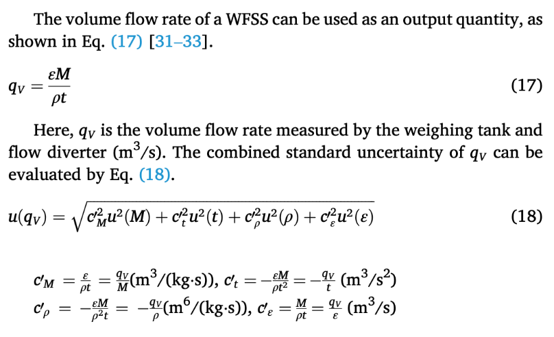
Sensitivity coefficients are defined in Equation (18) in the original article.Here, SC = , SC1 = /M, SC2 = -/t, SC3 = -/ρ, and SC4 = /ε.
q
V
q
V
q
V
q
V
q
V
Water-density formula (Tanaka / Patterson-Morris)
Water-density formula (Tanaka / Patterson-Morris)
Original notebook wrote this density expression out four times (about 160 lines) to form the finite differences drho2dT and drho2dP. Here, it is defined once as rho2[Tv, Pv]. The partial decomposition is preserved so the result is identical to the original:
drho2 = rho2[T0+dT, P0+dP] - rho2[T0, P0]
drho2 = rho2[T0+dT, P0+dP] - rho2[T0, P0]
Generation of random samples (Monte Carlo)
Generation of random samples (Monte Carlo)
Gaussian = NormalDistribution, rectangular = UniformDistribution (half-width = std*Sqrt[3]), Student-t = StudentTDistribution. A coverage factor of 2 (the level of confidence of approximately 95 %) is used downstream.
Density deviation via the single rho2 function (equivalent to the original 4 - block form)
Evaluate the CMC (reference flow rate)
Evaluate the CMC (reference flow rate)
Relative error e
Relative error e
Analysis #1: time series, histogram and Gaussian fit
Analysis #1: time series, histogram and Gaussian fit
Analysis #2: time series, histogram and Gaussian fit
Analysis #2: time series, histogram and Gaussian fit
◼
The Monte Carlo method generates the random signal of a measurand, e, to be investigated.
Summary of results
Summary of results
Optional check: distribution of t0
Optional check: distribution of t0
CITE THIS NOTEBOOK
CITE THIS NOTEBOOK
Validation of a large-capacity water flow standard system from (0.01 to 2000) m^3/h at KRISS
by Sejong Chun
Wolfram Community, STAFF PICKS, June 11, 2026
https://community.wolfram.com/groups/-/m/t/3732492
by Sejong Chun
Wolfram Community, STAFF PICKS, June 11, 2026
https://community.wolfram.com/groups/-/m/t/3732492