We assume that the flow rate is proportional to height of the tank and that the feed flow rate is constant equal to 1. This leads to a set of nonlinear ODEs that can only be solved numerically using NDSolve. We plot the height of both tanks versus time. In addition, we control of the height of the second tank (set point equal to 2) by manipulating the feed flow rate using proportional (P) and proportional - integral (PI) controllers. We plot for each case the height of both tanks and the feed flow rate versus time.
Assume volumetric flow rate proportional to square root of tank height : (t)=(t) where i=1, 2. Initially the two tanks are empty. Tank volume (t)=(t) for i=1..2.
q
i
k
i
h
i
v
i
A
i
h
i
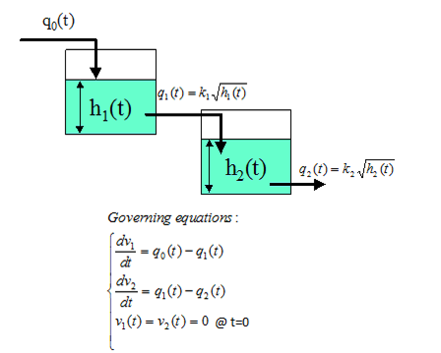
Feed flow rate is constant equal to 1
In[]:=
q
0
Numerical solution of the governing equations for =4, =3, =0.5and=1.2
A
1
A
2
k
1
k
2
In[]:=
A
1
A
2
k
1
k
2
In[]:=
sol1=NDSolve[t]-[t]D[[t],{t,1}],[t]-[t]D[[t],{t,1}],[0]0,[0]0,{[t],[t]},{t,0,1000}
q
0
k
1
h
1
A
1
h
1
k
1
h
1
k
2
h
2
A
2
h
2
h
1
h
2
h
1
h
2
Out[]=
[t]InterpolatingFunction[t],[t]InterpolatingFunction[t]
h
1


h
2

Plotting heights of the two tanks versus time
In[]:=
plt1=Plot[{[t]/.sol1,[t]/.sol1},{t,0,200},PlotStyle{Darker@Red,Darker@Green},AspectRatio1,GridLinesAutomatic,FrameTrue,ImageSize400{1,1},PlotRange{-0.1,5},FrameLabel{Style["time",14],Style["tank height",14]},PlotLegends{Style["tank 1",14],Style["tank 2",14]}]
h
1
h
2
Out[]=
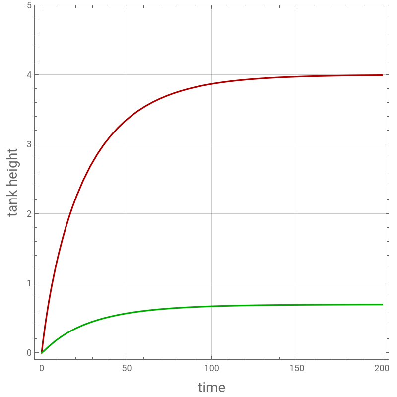


Control of the height of the second tank (set point equal to 2) by manipulating the feed flow rate using proportional and proportional-integral controllers.
Proportional controller gain =5
K
p
In[]:=
K
p
hset
2
Feed flow rate
In[]:=
q
0
K
p
hset
2
h
2
Numerical solution of the governing equations for =4, =3, =0.5and=1.2
A
1
A
2
k
1
k
2
In[]:=
sol2=NDSolve[t]-[t]D[[t],{t,1}],[t]-[t]D[[t],{t,1}],[0]0,[0]0,{[t],[t]},{t,0,1000}
q
0
k
1
h
1
A
1
h
1
k
1
h
1
k
2
h
2
A
2
h
2
h
1
h
2
h
1
h
2
Out[]=
[t]InterpolatingFunction[t],[t]InterpolatingFunction[t]
h
1

h
2

Plotting heights of the two tanks versus time
In[]:=
plt2=Plot[{[t]/.sol2,[t]/.sol2},{t,0,200},PlotStyle{Darker@Red,Darker@Green},AspectRatio1,GridLinesAutomatic,FrameTrue,ImageSize400{1,1},PlotRange{-0.1,15},FrameLabel{Style["time",14],Style["tank height",14]},PlotLegends{Style["tank 1",14],Style["tank 2",14]}]
h
1
h
2
Out[]=
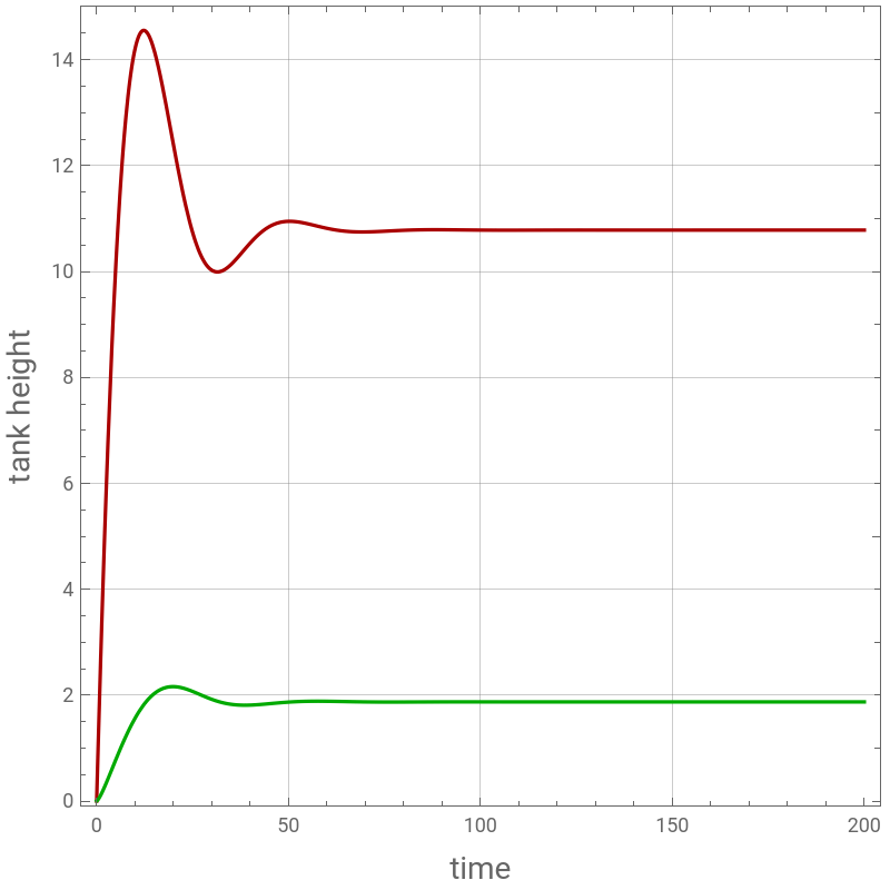
Plotting feed flow rate versus time
In[]:=
plt3=Plot[[t]/.sol2,{t,0,200},PlotStyleDarker@Blue,PlotRangeAll,AspectRatio1,GridLinesAutomatic,FrameTrue,ImageSize400{1,1},PlotRange{-0.1,5},FrameLabel{Style["time",14],Style["feed flow rate",14]}]
q
0
Out[]=
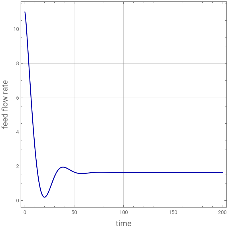
height of the second tank (with proportional only controller there is an offset)
offset = 2 - 1.872 = 0.128
offset = 2 - 1.872 = 0.128
In[]:=
h
2
Out[]=
{1.87166}
Proportional-integral controller gain =5 and time constant =20.
K
p
τ
I
In[]:=
K
p
hset
2
τ
I
Feed flow rate
In[]:=
q
0
K
p
hset
2
h
2
K
p
τ
I
Numerical solution of the governing equations for =4, =3, =0.5and=1.2
A
1
A
2
k
1
k
2
In[]:=
sol3=NDSolve[t]-[t]D[[t],{t,1}],[t]-[t]D[[t],{t,1}],D[int[t],{t,1}]-[t],[0]0,[0]0,int[0]0,{[t],[t],int[t]},{t,0,1000}
q
0
k
1
h
1
A
1
h
1
k
1
h
1
k
2
h
2
A
2
h
2
hset
2
h
2
h
1
h
2
h
1
h
2
Plotting heights of the two tanks versus time
height of the second tank
with proportional-integral controller the offset is removed but there is an overshoot and oscillations.
with proportional-integral controller the offset is removed but there is an overshoot and oscillations.
Plotting feed flow rate versus time
CITE THIS NOTEBOOK
CITE THIS NOTEBOOK
P and PI control of two tanks in series
by Housam Binous and Ahmed Bellagi
Wolfram Community, STAFF PICKS, July 20, 2023
https://community.wolfram.com/groups/-/m/t/2972951
by Housam Binous and Ahmed Bellagi
Wolfram Community, STAFF PICKS, July 20, 2023
https://community.wolfram.com/groups/-/m/t/2972951