Full version of the code here: https://www.wolframcloud.com/obj/yufanwang07/Published/aggregation_chaos.nb
Chaos theory explores the unpredictable and complex behavior of deterministic systems. Cellular automata (CA), as discrete mathematical models, can exhibit intricate patterns and behaviors despite simple rules. This essay investigates the presence of chaos theory within cellular automata aggregations and tilings. In this paper, we explore how multicomputational processes in cellular automata lead to chaotic behavior, the implications of such behaviors on understanding complex systems, and the potential applications of these insights.
Introduction
Introduction
Cellular automata (CA) are grid-based models used to simulate complex systems with simple, local rules. Each cell in the grid updates its state based on the states of its neighbors, leading to emergent behavior over time. Despite their simplicity, cellular automata can exhibit a wide range of behaviors, including periodicity, randomness, and chaos.
Out[]=
Some sample cellular automata |
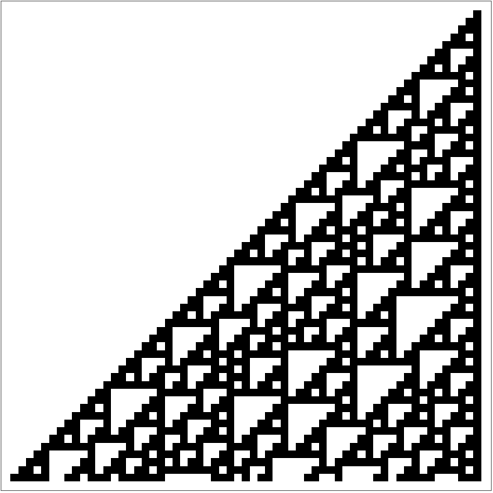
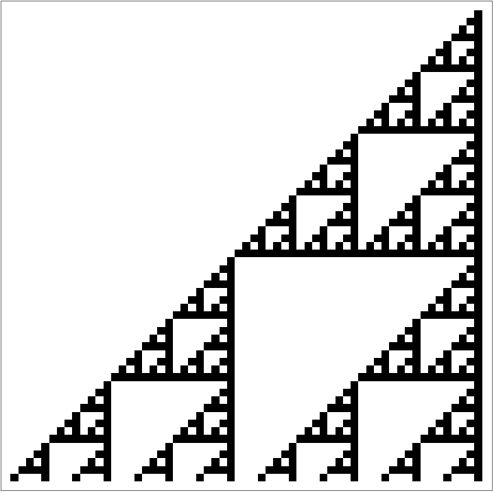
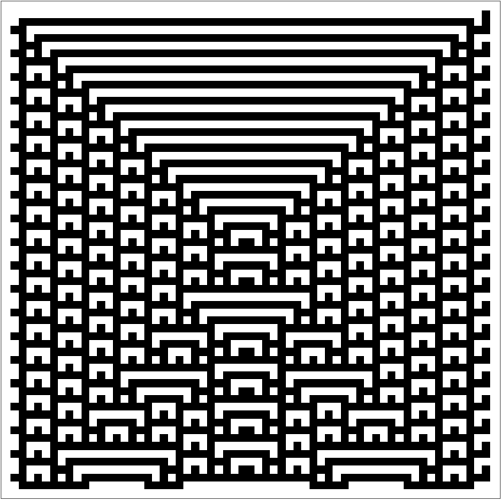
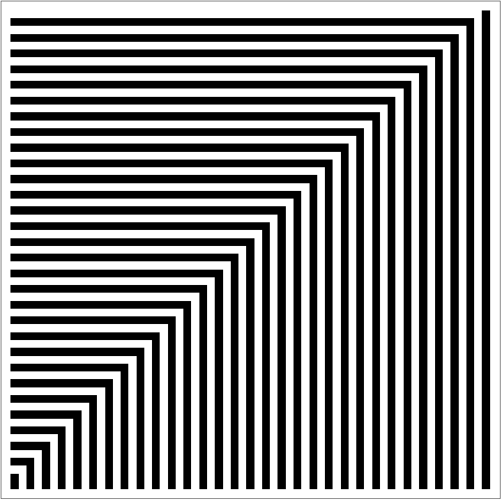
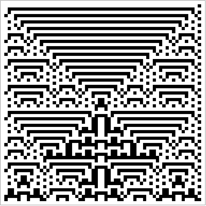
Chaos theory, introduced by Edward Lorenz in the 1960s, describes how deterministic systems can exhibit unpredictable and highly sensitive behavior. This sensitivity to initial conditions, often called the “butterfly effect,” is a hallmark of chaotic systems. For simplification purposes, we will start by dealing with the classical Eden growth model of aggregation; following Steven Wolfram’s example, we will aggregate by choosing a new tile at random that satisfies existing conditions. For instance, here’s what the case for the rule of any bordering tile may give:
In[]:=
trimZeroEdges[array_] := Module[{trimmedArray = array}, While[First[trimmedArray] === ConstantArray[0,Length[First[trimmedArray]]], trimmedArray = Rest[trimmedArray]]; While[Last[trimmedArray] === ConstantArray[0,Length[First[trimmedArray]]], trimmedArray = Most[trimmedArray]]; trimmedArray = Transpose[trimmedArray]; While[First[trimmedArray] === ConstantArray[0,Length[First[trimmedArray]]], trimmedArray = Rest[trimmedArray]]; While[Last[trimmedArray] === ConstantArray[0,Length[First[trimmedArray]]], trimmedArray = Most[trimmedArray]]; Transpose[trimmedArray]]
In[]:=
centerPad[array_, size_] := Module[{rows, cols, padTop, padBottom, padLeft, padRight}, {rows, cols} = Dimensions[array]; padTop = Ceiling[(size - rows)/2]; padBottom = size - rows - padTop; padLeft = Ceiling[(size - cols)/2]; padRight = size - cols - padLeft; ArrayPad[array, {{padTop, padBottom}, {padLeft, padRight}}, 0]]
Out[]=



We can also only append to tiles with a fixed number of surrounding alive cells. The following case shows the case where only cells with two surrounding alive tiles are aggregated:
Out[]=
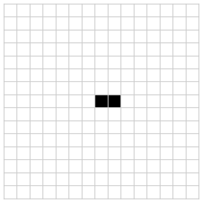
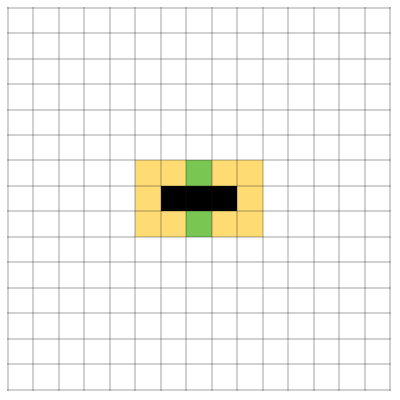
And similarly for three (see left diagram below); we will refer to this aggregation rule from now on as rule {3}. Additionally, for the rest of this paper, we’ll deal with the latter case: only cells with exactly three surrounding alive tiles can be aggregated. For ease of visualization, we’ll colorize bordering tiles according to the following legend: black tiles will be alive, and white tiles will be ones not currently aggregated. Orange tiles are tiles that cannot be tiled, as the number of surrounding aggregated tiles exceeds 3. Yellow tiles are those that do not yet have sufficient surrounding tiles to be aggregated yet, but may have enough in the future. Lastly, green tiles are those that can be aggregated, having exactly three surrounding tiles. The identical coloring is provided on the right.

Out[]=
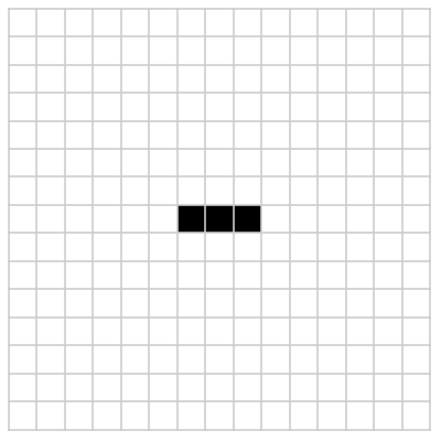
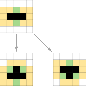
We can model the step-by-step formation of these aggregations using multiway graphs, with a source state connecting to the tilings it can aggregate to. For instance, using the same rule, a single step of the aggregation may look like the below:
In[]:=
Prettify[graph_] := ImageCrop[Show[graph]]
In[]:=
AggregationMultiway[rule_, depth_, canonicalize_ : True, start_ : {{0, 1}, {0, 0}, {0, -1}}] := Graph[{3}] {3},[2,8], start, depth, "Canonicalize" -> canonicalize, ColorRules -> ["GrowthColors", "Light"], "Boundary"->True, Mesh->None, EdgeStyle->Gray, VertexSize->1.3, GraphLayout->"LayeredDigraphEmbedding", ImageSize->{Automatic,250}
Out[]=
We can take this further; the same multiway graph for depth 3 is shown below.
Out[]=
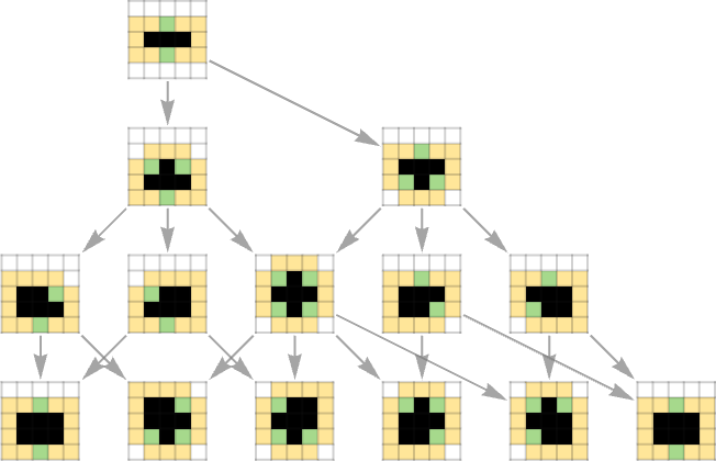
We note that a lot of the intermediate steps are identical: for instance, the middle four leaf nodes are simply rotations of one another. We can account for differences in rotations and translations in creating out multiway graph.
Out[]=
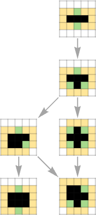
We will use these multiway graphs of aggregation systems as the primary visualization of their properties. Multiway graphs can quickly expand beyond bound; a multiway graph of the above with depth 17 is shown below:
Out[]=
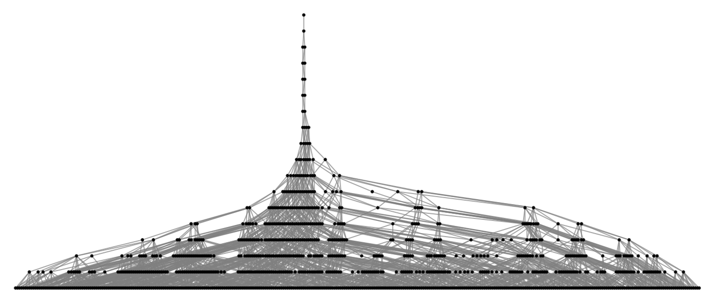
In these cases, the graph becomes so chaotic that it becomes difficult to see any sort of structured pattern. However, we can utilize embeddings to help create a more structured diagram:
We may also potentially find solutions in higher dimensions.
Terminal States and Their Multiway Instability
Terminal States and Their Multiway Instability
According to convention, we will refer to a state where no further aggregations are possible a “terminal state.” Terminal states can be seen visually as a leaf on a multiway graph—a node without children. Clearly, terminal states differ for a variety of aggregation rules; for our rule {3}, a few select terminal states are shown below.
It is easy to see that these terminal states are only somewhat stable. We will say that a state can “break free” if its aggregation multiway graph can expand significantly beyond its original depth. Visually, in this example, we can see that backtracking one step from a terminal state in the multiway graph always allows for said terminal state to “break free,” with there being a path to continue expanding. If we restrict ourselves to only the above terminal states, assuming a random choice, backtracking one step results in a 50%, 50%, and 33.3% chance to break free, respectively. The first step of said paths are shown below—one can continue by selecting any non-highlighted follow-up path.
We can go one step further by removing the constraint on “legal operations” and allowing choices outside existing edges. We will again work with the left-most terminal state.
This terminal state is found in the multiway diagram above as the right-most element in the boxed zone. As mentioned before, the chance of breaking free by backtracking one step is 33.3%. Removing one tile on the border can result in any of the following:
We can then create multiway graphs with each of these as a root, which gives us the following.
And connecting each of these to the same starting root as a general multiway graph results in the below.
The structure of this instability may be visualized in a different embedding.
Compiling terminal probabilities gives a surprisingly similar result: out of the 16 states removing a bordering tile leads to, only 5 break free, giving a total of 31.25%, a value suspiciously close to our previous value of 33.3%. However, this is a little unfair—a large portion of our terminal states are the result of making an implausible change, resulting immediately in another terminal state (visually demonstrated in the large quantity of leaf nodes in the first radial ring above). Removing these cases from our total results in a much more balanced 45.5%. A similar experiment could be done on larger terminal states, and for a similar result.
False Stability in Terminal States
False Stability in Terminal States
Now that we somewhat understand the instability of terminal states, we have a position to stat exploring chaos theory. We will start with a configuration bigger than our previous initial aggregation to emphasize effects of an initial perturbation. The code used to generate the initial setups was a brute force program which iterated over every possible iteration up to iteration depth 5000 and checks if every outgoing path converges to a terminal state in depth 3. The program ran overnight, generating 2.9 GB of solutions (part of the reason said data isn’t included in this notebook). The initial aggregation is shown below.
Here’s the multiway graph for the above:
We can make one small change to the border of the original starting aggregation position. Note that we only need to consider the border—any change in the internal structure will only be confined to the internal content. Here’s the edited version of the starting position:
Note the one-block difference on the top arm. We will now plot the multiway graph for the new starting aggregation.
We can see that the single block change has fundamentally changed how growth can occur—we see an explosion of growth in the section where the modified arm is present. Here’s the same multiway graph, iterated to a higher depth:
Here’s the above in a three-dimensional embedding.
Note that the non-modified subgraph is actually present in the expansive multiway graph: here’s a depiction of the two graphs side by side, with the terminal one highlighted in the modified one.
What we are doing here is essentially backtracking one step through the aggregation multiway graph and retrying the step that led to a terminal state.
Quantifying the Propagation of Chaos in Terminal States
Quantifying the Propagation of Chaos in Terminal States
A direct comparison of two initial states are also possible. We can sum over differences throughout each aggregation step, and plot differences over time—we will refer to this “chaos” score from now on as the accumulated divergence. For sake of simplicity, we will first use the Euclidean distance between two aggregation positions. This can be implemented in the following way:
We will first check some edge cases. A commparison of two identical tilings is shown below.
As expected, if we use the exact same processes, we will see no difference; and hence no accumulated divergence. We will now compare the modified and non-modified versions:
However, the current measure of accumulated divergence is not quite optimal: a graph for two random different aggregations with the same starting position a similar curve:
We can certainly improve our measure of accumulative divergence by instead aggregating the differences between the Euclidean distance from the origin to the aggregated point. We can change our implementation slightly to account for the new formula:
Using this technique, our modified terminal aggregation becomes:
With a very similar result to the previous aggregation. However, our random distribution becomes much different:
Now, with the new definition of accumulative divergence, we see a somewhat parabolic relationship for the terminal condition and a near-linear relationship for random generation. This makes sense—the butterfly effect causes divergence over time, while random aggregation will add approximately the same amount to the score each time. It makes sense to subtract the random condition from the original to in a sense “remove” the effect of random aggregation, and leave us with purely the effect of instability. We implement this by making a minor change once more to the formula:
Here’s the result upon subtracting the effect of randomness.
The diagram now seems to fluctuate more than before, but still resembles the general parabolic shape, as seen before. To visually show the effect of the change, we could aggregate both tilings to some large depth. For instance, in the following diagram, the left side is the original aggregation iterated (to a terminal state), while the right side is shown at a depth 5000.
One can find the original tiling in the right hand diagram—look right above the bulge section on the left side.
The Lyapunov Exponent for Discrete Systems
The Lyapunov Exponent for Discrete Systems
We now attempt to quantify this propagation of chaos. The Lyapunov Exponent is a commonly used concept to measure the presence of chaos and instability in continuous systems, quantifying the rate at which nearby trajectories diverge in a dynamical system. However, it is certainly possible to extend this to discrete systems such as cellular automata and aggregation tilings as mentioned above. Work has already been done on measuring the Lyapunov Exponent for 1-dimensional cellular automata. However, we don’t have to take nearly as complicated an approach as the existing work. In the previous section, we managed to derive various graphical representations of the accumulative divergence. We can fit this to the formula for the Lyapunov exponential model. We start by generating the data involved:
Something strange occurs: when we try to fit t his to an exponential function as below, we cannot find a fitting of sufficient accuracy (the red line below is the fitted exponential function):
However, this can be explained—our single-tile aggregation holds little meaning, as the rate of growth of aggregation is far too small to allow for exponential change. Taking this into account, and using the exponential of the root of x instead of x directly gives us a much more promising result:
Indeed, plotting this shows an almost perfect match:
From this, we can then conclude that the Lyapunov exponent for our above system is approximately 0.132. A positive Lyapunov exponent indicates chaos, where small differences in initial conditions lead to exponentially divergent outcomes. Conversely, a negative or zero Lyapunov exponent suggests stability, where trajectories converge or remain equidistant over time. Our value of 0.132 suggests a divergent, though only modestly chaotic aggregation. We can try modeling this for other aggregations as well:
We can extract the accumulative divergence data at each step:
We fit the model once again:
And plotting this gives a decent fit.
The curve does not fit to the data nearly as well as before, due to our expansion to a depth of 3500 and a drastic increase of data points. However, the graph is still exponential in shape—this time, with a Lyapunov exponent of 0.0646. The exponent remains positive, however, suggesting that divergent effects of chaos are still present.
Note on the General Aggregation {n}
Note on the General Aggregation {n}
Throughout the course of this paper, we have done simulations, calculations, and research only in the scope of the aggregation rule {3}. However, the results involved are not constrained to this case—we focused simply on rule {3} due to its convenient amount of convergence, ease of computation, and simplicity. To demonstrate this, a brief exploration for rule {2} is shown below. We start by generating terminal states:
We will work with this following initial position:
We generate the boundary tiles as before:
Note that due to the structure of terminal states for rule {2}, there are a lot more of what we consider “boundary tiles.” We can draw multiway graphs for each one, then compile them into a single graph to demonstrate the same effects as before:
We see that this case is even more unstable than the last—a majority of the cases manage to break free, with all the remaining ones being ones we eliminated being terminal states. Again, a different embedding may be helpful:
Something similar could be done for other rules as well.
Implications and Applications
Implications and Applications
Understanding chaos in cellular automata and aggregation systems has significant implications for various fields, including computer science, physics, and biology. The study of chaotic behavior in these systems can inform the design of algorithms for solving complex problems, modeling natural phenomena, and developing robust artificial intelligence systems.
Specifically, aggregation systems such as the explored Eden model have applications to aspects of aggregator cellular growth such as tumor growth. A study into perturbation of initial conditions could potentially be beneficial in the treatment of such processes.
Specifically, aggregation systems such as the explored Eden model have applications to aspects of aggregator cellular growth such as tumor growth. A study into perturbation of initial conditions could potentially be beneficial in the treatment of such processes.
Conclusion
Conclusion
The exploration of chaos theory within cellular automata aggregations and tilings provides a rich framework for understanding the emergence of complexity from simplicity. By examining the multicomputational processes in cellular automata, we gain valuable insights into the nature of chaos and its implications for various scientific and practical applications. Wolfram’s work on cellular automata serves as a foundation for further research into the intricate and fascinating world of chaotic systems. The ability to quantify these aggregation systems with conventional methods such as Lyapunov exponentiation suggests a deeper reliance upon foundations of chaos theory.
Future Directions
Future Directions
During the writeup of this paper, when creating code for visualizations, I stumbled upon the phenomena that for rule {3} the chance of a state breaking free, using legal and non-legal moves, are both roughly 1/3. Additionally, in the expansion into rule {2}, the chance of a state breaking free is roughly 1/2. This may be nothing more than a coincidence, but is definitely something I aim to explore in the future. Additionally, it may be possible to generate predictions of future aggregations through recognition of substructures.
Acknowledgements
Acknowledgements
Thank you to my mentor Dugan Hammock for aiding me in the completion of this project. Thank you to the TAs at WSRP, the directors for providing us with this experience, and Steven Wolfram for the foundations of this project, in more ways than one.
References
References
1
.Stephen Wolfram (2023), “Aggregation and Tiling as Multicomputational Processes,” Stephen Wolfram Writings. https://writings.stephenwolfram.com/2023/11/aggregation-and-tiling-as-multicomputational-processes
2
.Wolfram, Stephen. A New Kind of Science. Wolfram Media, 2002, Champaign, IL. ISBN 1-57955-008-8. Published May 14, 2002. Available at: www.wolframscience.com
3
.Jan Baetens, “Lyapunov Exponents of Elementary Cellular Automata,” Wolfram Demonstrations Project. https://demonstrations.wolfram.com/LyapunovExponentsOfElementaryCellularAutomata/
4
.Weisstein, Eric W. “Lyapunov Characteristic Exponent.” From MathWorld--A Wolfram Web Resource. https://mathworld.wolfram.com/LyapunovCharacteristicExponent.html
5
.“Lyapunov Exponent.” Wikipedia, 8 July 2023, https://en.wikipedia.org/wiki/Lyapunov_exponent. Accessed 11 July 2024.
CITE THIS NOTEBOOK
CITE THIS NOTEBOOK
On chaos in aggregation systems
by Yufan Wang
Wolfram Community, STAFF PICKS, July 12, 2024
https://community.wolfram.com/groups/-/m/t/3215676
by Yufan Wang
Wolfram Community, STAFF PICKS, July 12, 2024
https://community.wolfram.com/groups/-/m/t/3215676