The Bass diffusion model is modified (1) to include the total number of potential customers and (2) to clarify the meaning of the model which did not use usual notations.
Introduction
Introduction
◼
Frank Bass developed a model to describe how new products get adopted in a population. This mode l has been widely used.
◼
f[t]
1-F[t]
◼
F[t] is the installed base fraction, that is, F[t] represents the cumulative number of people who adopt a new product.
◼
f[t] is the change of the installed base fraction, i.e.,
f[t]=F[t]
t
◼
“p” is the coefficient of innovation, that is, (1) technological innovation will make people to adopt a new product and it is also known as technological push
◼
“q” is the coefficient of imitation, that is, (2) People adopt a new product by world of mouth and it is also termed as customers’ pull.
Re-arranged Bass diffusion model
Re-arranged Bass diffusion model
◼
The Bass model looks strange so I re-arranged the Bass diffusion model for easy understanding by moving the denominator .
◼
f(t)=F[t]={p+qF(t)}-{pF(t)+q}=inflow-outflow
t
2
F(t)
◼
Key point: The revised equation shows two factors for inflow,{p+q F(t)}, and two factors for outflow. Note that the outflow has the square term, , therefore p* will be quickly larger than the inflow of q*F[t], reaching to its steady state. This is very similar to the logistic differential equation, where f[t]=f[t]-.
2
F[t]
2
F[t]
t
2
f[t]
◼
Inflows:
p+qF(t)
◼
Outflows:
-pF(t)-q
2
F(t)
In[]:=
(*re-arrancetheBassmodel,showinginflowswithpositivesignandoutflowswithnegativesigns*)Solve[f[t]/(1-F[t])p+q*F[t],f[t]]//Expand
Out[]=
{{f[t]p-pF[t]+qF[t]-q}}
2
F[t]
Bass diffusion model with total number of customers
Bass diffusion model with total number of customers
◼
I introduce a new variable “m” that represents the total number of potential customers who will adopt a product(f1[t]) and changed notations(f2[t]).T the “m” is usually normalized to 1 or 100% but the “m” can be set to other values.
◼
f
1
◼
f
2
◼
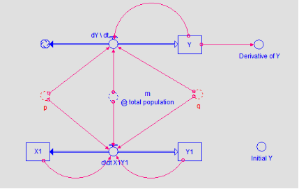
Y[t]=F[t]. Y[t] represent the cumulative number of adopters
◼
X[t]=1-F[t] . X[t] represents the number of potential customers
◼
Stock-Flow diagram
Out[]=
◼
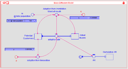
e.g., Interpretation
◼
p*PotentialCustomers(t)+(q/m)*PotentialCustomers(t)*ActualBuyers(t)
Modeling
Modeling
In[]:=
psol=ParametricNDSolve[{x'[t]-(p*x[t]+(q/m)*x[t]*y[t]),y'[t](p*x[t]+(q/m)*x[t]*y[t]),x[0]m,y[0]0},{x,y},{t,0,100},{p,q,m}]
Out[]=
xParametricFunction,yParametricFunction


Simulation
Simulation
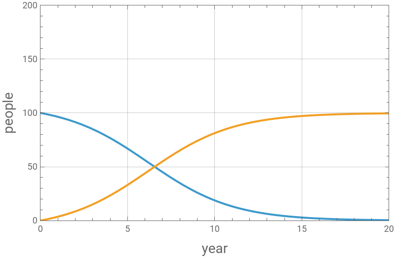
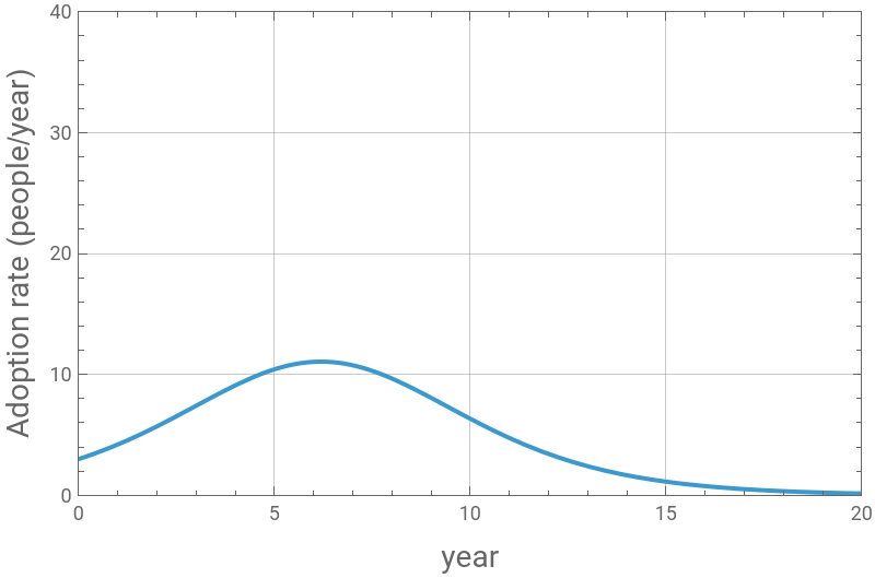
The default values for p and q are from the meta analysis of literature reviews. The average values of p and q have been found to be 0.03 and 0.38, respectively.
In[]:=
Manipulate[Row[{Plot[Evaluate[{x[p,q,m][t],y[p,q,m][t]}/.psol],{t,0,20},Frame->True,FrameLabel->{Style["year",14],Style["people",14]},PlotLegends->Placed[{"No. of Potential Customers","No. of Adopters"},Above],GridLines->Automatic,ImageSize400,PlotRange{{0,20},{0,200}}],Plot[Evaluate[{y[p,q,m]'[t]}/.psol],{t,0,20},Frame->True,FrameLabel{Style["year",14],Style["Adoption rate (people/year)",14]},PlotLegendsPlaced[{"Adoption rate (people/year)"},Above],GridLines->Automatic,ImageSize400,PlotRange{{0,20},{0,40}}]}],{{p,0.03,Style["p = coefficient of innovation",14]},0.00,0.5,0.01},{{q,0.38,Style["q = coefficient of imitation",14]},0.00,0.5,0.01},{{m,100,Style["Total potential customers",14]},0,200,10},SaveDefinitions->True]
Out[]=


Observation and Discussion
Observation and Discussion
◼
Findings
◼
“p” makes the adoption rate curve move left or write)
◼
“q” makes the adoption rate curve be narrow or wide
◼
The bass diffusion model is one of the most widely used model but this model does not explain what causes people to adopt and to innovate: status symbol, early-adopters, etc. P and q are used as an exogenous parameters (that is, they are just given)
◼
What drives the p and q? price
◼
It is shown that the bass diffusion model is accurate if 50% of lifetime data are once available to fit, in other words, half of the life cycle (need to find out the reference). Therefore this is a good model to fit the adoption rate once lots of data are available, but ......
◼
useful planning tool? How do we estimate the values of p and q well in advance when a new product is just released such as electrical vehicle? It might be too late if we wait until the 50% of life time data are to be available....because the uncertainty in estimating p and q value will result in wide ranges of adopters as well as the adoption rate......
Appendix
Appendix
Bass diffusion model using the f1[t]
Bass diffusion model using the f1[t]
f1(t)=p*(100-F(t))+(q/m)*(100-F[t])*F(t)
In[]:=
psol3=ParametricNDSolve[{F'[t]p*(100-F[t])+(q/m)*(100-F[t])*F[t],F[0]0.0}(*F[t]representthecumulativenumberofpeoplewhoadoptedaproduct*),{F},{t,0,100},{p,q,m}]
◼
F[t] represents the cumulative number of people who adopted a product. Thus 1 - F[p,q,m][t] is the number of potential customers.
Bass diffusion model in original equation
Bass diffusion model in original equation
◼
F[t] represents the cumulative number of people who adopted a product. Thus 1 - F[p,q,m][t] is the number of potential customers.