ABSTRACT (original article): In 1966, Leo Moser introduced the ”moving sofa problem,” which seeks to determine the largest area of a shape that can be maneuvered through a 90-degree hallway of unit-width. This problem remains unsolved and open yet. In this paper, we employ calculus of variations method. Assuming the trajectories and envelopes are convex, the sofa’s area is formulated as an integral functional on a set of parametric equations for curves. The final shape is determined by solving the Euler-Lagrange equations. Utilizing numerical methods, we obtain the non-trivial area of 2.2195316, consistent with the previously well-known Gerver’s constant since 1992. We prove that the results of Gerver’s sofa satisfies the Euler-Lagrange equations for the necessary condition of maximal area. CITATION (original article): Zhipeng Deng (2024), Solving Moving Sofa Problem Using Calculus of Variations, arXiv:2407.02587. https://doi.org/10.48550/arXiv.2407.02587
Details of methods, equations, assumptions, more results, and further discussions can be found in the paper https://arxiv.org/abs/2407.02587
Calculus of variations for type of Gerver’s sofa
Calculus of variations for type of Gerver’s sofa
To formulate the problem, we first create a 2D coordinate system as shown below. We assume the sofa shape rotates and moves clockwise, equivalent to the hallway wall rotating counterclockwise. Thus, lines AB, AC, ApBp, and ApCp rotate counterclockwise.
ShowTableListLinePlot{r*Cos[a],t*Sin[a]},r*Cos[a]-,0,{{r*Cos[a],t*Sin[a]},{r*Cos[a]+t*Sin[a]*Tan[a/2],0}},r*Cos[a]+-,0,r*Cos[a]+,0/.{r->0.2,t->0.2},,{a,0,0.3π,0.3π},PerformanceGoal->"Speed"//Quiet
t*Sin[a]
Tan[a/2]
2
*Cos[π/4+a/2],t*Sin[a]+2
*Sin[π/4+a/2],r*Cos[a]-t*Sin[a]
Tan[a/2]
1
Sin[a/2]
2
*Cos[π/4+a/2],t*Sin[a]+2
*Sin[π/4+a/2],r*Cos[a]+t*Sin[a]*Tan[a/2]+1
Cos[a/2]
Out[]=
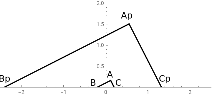
Moving sofa in a hallway with unit width, we assume the hallway has a lower edge along the X-axis y = 0, and the upper edge along the line y = 1.
We employ parametric equations with two functions r(α) and t(α) to define a family of curves to be determined, where α represents the rotation angle with 0 ≤α ≤π. These curves are assumed to be differentiable and well-behaved.
We employ parametric equations with two functions r(α) and t(α) to define a family of curves to be determined, where α represents the rotation angle with 0 ≤α ≤π. These curves are assumed to be differentiable and well-behaved.
The coordinates of the points are defined as follows
In[]:=
AA={r[α]*Cos[α],t[α]*Sin[α]};AAp=r[α]*Cos[α]+,0};BBp={r[α]*Cos[α]-t[α]*2-1Sin[α/2],0};CC={r[α]*Cos[α]+t[α]*Sin[α]*Tan[α/2],0};CCp={r[α]*Cos[α]+t[α]*Sin[α]*Tan[α/2]+1/Cos[α/2],0};EAABBx=1/2*(-1+2Cos[α]+Cos[2α])r[α]-2Cos[α]t[α]+Sin[α](Cos[α]r'[α]-(1+Cos[α])t'[α]);EAABBy=-2(r[α]Sin[α]-Sin[α]t[α]-Cos[α]r'[α]+t'[α]+Cos[α]t'[α]);EAACCx=r[α](Cos[α]+)-2Cos[α]t[α]+Sin[α](-Cos[α]r'[α]+(-1+Cos[α])t'[α]);EAACCy=2(-r[α]Sin[α]+Sin[α]t[α]+Cos[α]r'[α]+t'[α]-Cos[α]t'[α]);EAApBBpx=1/2*((-1+2Cos[α]+Cos[2α])r[α]-2Sin[α/2]-4Cos[α]t[α]+Sin[2α]r'[α]-2Sin[α]t'[α]-Sin[2α]t'[α]);EAApBBpy=1/2*(2Cos[α/2]+r[α](-2Sin[α]+Sin[2α])-2(-1+Cos[α])Sin[α]t[α]-r'[α]+2Cos[α]r'[α]-Cos[2α]r'[α]-t'[α]+Cos[2α]t'[α]);EAApCCpx=1/2*(2Cos[α/2]+2r[α](Cos[α]+)+(1-2Cos[α]+Cos[2α])t[α]-Sin[2α]r'[α]-2Sin[α]t'[α]+Sin[2α]t'[α]);EAApCCpy=1/2*(2Sin[α/2]-2(1+Cos[α])r[α]Sin[α]+(2Sin[α]+Sin[2α])t[α]+r'[α]+2Cos[α]r'[α]+Cos[2α]r'[α]+t'[α]-Cos[2α]t'[α]);
2
*Cos[π/4+α/2],t[α]*Sin[α]+2
*Sin[π/4+α/2];BB={r[α]*Cos[α]-t[α]*22
Cos[α/2]
2
Cos[α/2]
2
Cos[α/2]
2
Sin[α/2]
2
Sin[α]
2
Sin[α/2]
2
Cos[α/2]
2
Cos[α/2]
2
Sin[α]
Assume intersection point was p for trajectory of point A and AC envelope
AA[[1]] /. α -> α1p == EAACCx /. α -> α2p
AA[[2]] /. α -> α1p == EAACCy /. α -> α2p
AA[[1]] /. α -> α1p == EAACCx /. α -> α2p
AA[[2]] /. α -> α1p == EAACCy /. α -> α2p
Assume approximate values of α1 and α2 for piecewise function
In[]:=
α1p=77/1000;
In[]:=
α2p=177/100;
Define integral functional for sofa area
FF=Piecewise[{{0,α<0},{-(EAApBBpx/.α->0)-EAApBBpy*D[EAApBBpx,α]-EAApCCpy*D[EAApCCpx,α]-EAABBy*D[EAABBx,α],0<=α<=α1p},{-(EAApBBpx/.α->0)-EAApBBpy*D[EAApBBpx,α]-EAApCCpy*D[EAApCCpx,α]+AA[[2]]*D[AA[[1]],α]-EAABBy*D[EAABBx,α],α1p<α<=1},{-EAApBBpy*D[EAApBBpx,α]-EAApCCpy*D[EAApCCpx,α]+AA[[2]]*D[AA[[1]],α]-EAABBy*D[EAABBx,α],1<α<=π-α2p},{-EAApBBpy*D[EAApBBpx,α]-EAApCCpy*D[EAApCCpx,α]+AA[[2]]*D[AA[[1]],α],π-α2p<α<=π/2},{0,π/2<α}}]//Simplify;
Euler–Lagrange equations in calculus of variations
In[]:=
(D[FF,r[α]]-D[D[FF,r'[α]],α]+D[D[FF,r''[α]],{α,2}])//Simplify
Out[]=
|
In[]:=
(D[FF,t[α]]-D[D[FF,t'[α]],α]+D[D[FF,t''[α]],{α,2}])//Simplify
Out[]=
|
Use internal package and function to obtain the same Euler–Lagrange equations
In[]:=
Needs["VariationalMethods`"]
In[]:=
EulerEquations[FF,{r[α],t[α]},α]//Simplify
Out[]=
α<0||0<α<&&Cos[α]-Cos-2(-3Cos[α]+Cos[2α])r[α]+Sin+2(-3Cos[α]+Cos[2α])t[α]+12Sin[α][α]-3Sin[2α][α]-6Sin[α][α]+3Sin[2α][α]+[α]-6Cos[α][α]+Cos[2α][α]+[α]-Cos[2α][α]0||1000α>77&&+α<π&&Cos[α]-Cos-2(-3Cos[α]+Cos[2α])r[α]+Sin+2(-2Cos[α]+Cos[2α])t[α]+12Sin[α][α]-3Sin[2α][α]-4Sin[α][α]+3Sin[2α][α]+[α]-6Cos[α][α]+Cos[2α][α]+[α]-Cos[2α][α]0||+α>π&&2α<π&&Cos[α]-Cos+4Cos[α]r[α]+Sin-2Cos[α]t[α]+8Sin[α][α]-2Sin[α][α]-4Cos[α][α]0||2α>π,α<0||0<α≤&&Sin[α]Cos+Sin+2r[α](3Sin[α]+Sin[2α])-2(3Sin[α]+Sin[2α])t[α]+[α]-6Cos[α][α]-3Cos[2α][α]+[α]+12Cos[α][α]+3Cos[2α][α]-Sin[2α][α]+6Sin[α][α]+Sin[2α][α]0||1000α>77&&+α<π&&Sin[α]Cos+Sin+4(1+Cos[α])r[α]Sin[α]-2(3Sin[α]+Sin[2α])t[α]+[α]-4Cos[α][α]-3Cos[2α][α]+[α]+12Cos[α][α]+3Cos[2α][α]-Sin[2α][α]+6Sin[α][α]+Sin[2α][α]0||+α>π&&2α<π&&Sin[α]Cos+Sin+2r[α]Sin[α]-4Sin[α]t[α]-2Cos[α][α]+8Cos[α][α]+4Sin[α][α]0||2α>π
77
1000
α
2
α
2
′
r
′
r
′
t
′
t
′′
r
′′
r
′′
r
′′
t
′′
t
177
100
α
2
α
2
′
r
′
r
′
t
′
t
′′
r
′′
r
′′
r
′′
t
′′
t
177
100
α
2
α
2
′
r
′
t
′′
r
77
1000
α
2
α
2
′
r
′
r
′
r
′
t
′
t
′
t
′′
r
′′
t
′′
t
177
100
α
2
α
2
′
r
′
r
′
r
′
t
′
t
′
t
′′
r
′′
t
′′
t
177
100
α
2
α
2
′
r
′
t
′′
t
Boundary condition for α = 0
In[]:=
FF0=-(EAApBBpx/.α->0)-EAApBBpy*D[EAApBBpx,α]-EAApCCpy*D[EAApCCpx,α]-EAABBy*D[EAABBx,α];
In[]:=
(D[FF0,r'[α],α]-D[D[FF0,r''[α],α],α])/.α->0
Out[]=
-+2r[0]-2t[0]-2[0]
1
2
′′
r
In[]:=
(D[FF0,t'[α],α]-D[D[FF0,t''[α],α],α])/.α->0
Out[]=
0
Numerical calculation
Numerical calculation
Initial guess of α1p
α1p=0.078;
Initial guess of α2p
α2p=1.78;
Numerical search for optimal boundary value t[0]
t0=0.7103;
Initial value for solving r[α]
ri=0.61;
Number of discretization points
pts=2001;
Discretization: αα is discrete parameter
αα=Range[0.,π/2,(π/2-0.)/(pts-1)];
Discretization setting of finite difference method with 4th difference order
dfdα=NDSolve`FiniteDifferenceDerivative[{1},{αα},"DifferenceOrder"4]["DifferentiationMatrix"];d2fdα2=NDSolve`FiniteDifferenceDerivative[{2},{αα},"DifferenceOrder"4]["DifferentiationMatrix"];
Find α1p and α2p iteratively
Calculate sofa area
Small error of 4 e - 8 from Gerver’ s 2.21953166 was due to approximate boundary values, discretization, and interpolation
Obtained α1p α2p
Display sofa shape
Display sofa shape with wall lines and envelop curves
Obtained parametric equations r (α), t (α)
Verify Gerver’ s results from previous paper
Verify Gerver’ s results from previous paper
Romik’ s explicit results from previous paper and code, explicit expression, code from movingsofas - v1 .3
https://www.math.ucdavis.edu/~romik/data/uploads/software/movingsofas-v1.3.nb
https://www.math.ucdavis.edu/~romik/data/uploads/software/movingsofas-v1.3.nb
Verify Gerver’ s and Romik’ s results satisfy E - L equations ODE1 and ODE2 when 0 < α < α1p
{0, 0} indicated Gerver’ s and Romik’ s results satisfy E - L equations!
Verify Gerver’ s and Romik’ s results satisfy satisfy E - L equations ODE1 and ODE2 when α1p < α <= π - α2p
Verify Gerver’ s and Romik’ s results satisfy E - L equations ODE1 and ODE2 when π - α2p < α <= π/2
CITE THIS NOTEBOOK
CITE THIS NOTEBOOK
Calculus of variation approach and Euler - Lagrange equations for the moving sofa problem
by Zhipeng Deng
Wolfram Community, STAFF PICKS, July 25, 2024
https://community.wolfram.com/groups/-/m/t/3234695
by Zhipeng Deng
Wolfram Community, STAFF PICKS, July 25, 2024
https://community.wolfram.com/groups/-/m/t/3234695