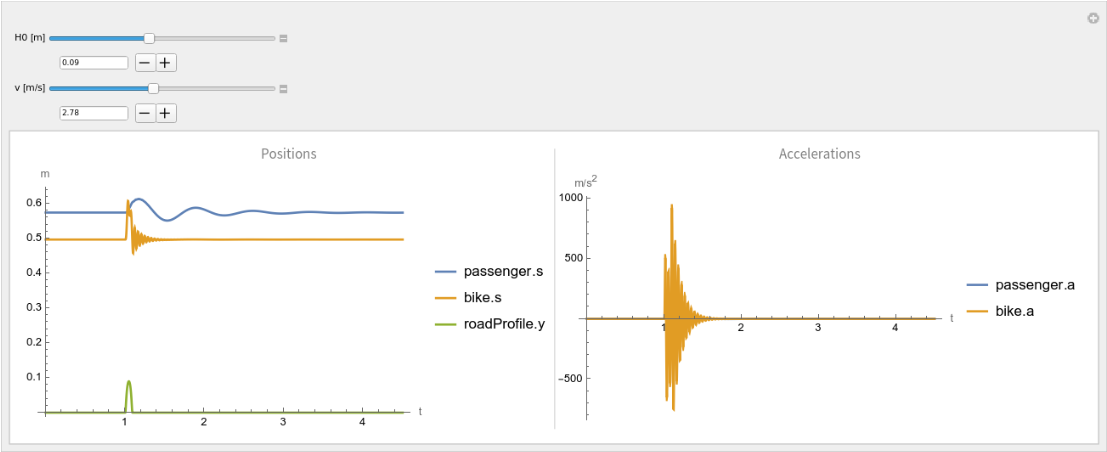
Let me start with a variation of the problem that has unstretched lengths for the springs, adds gravity and starts the system from the equilibrium positions (so as to reproduce the general behavior of your problem):
In[]:=
m1=50;(*kg*)m2=8;(*kg*)k1=4000;(*N/m*)k2=180000;(*N/m*)c=150;(*N×s/m*)z=2.71828;H0=0.09;(*m*)L0=0.27;(*m*)v=2.78;(*m/s*)l1=0.2;(*m,unstretchedspringlengthforspring1*)l2=0.5;(*m,unstretchedspringlengthforspring2*)g=9.8;(*m/,gravitationalacceleration*)timeStop=4.5;(*s,simulationstoptime*)h[t_]=
;
2
s
|
Solve for positions, velocities and accelerations together (instead of solving only for position and differentiating afterwards):
In[]:=
sol=FirstNDSolveax[t]==vx'[t],ay[t]==vy'[t],vx[t]==x'[t],vy[t]==y'[t],m1ax[t]+c(vx[t]-vy[t])+k1(x[t]-y[t]-l1)+m1g==0,m2ay[t]-c(vx[t]-vy[t])-k1(x[t]-y[t]-l1)+k2(y[t]-h[t]-l2)+m2g==0,x[0]==l1+l2--,vx[0]==0,y[0]==l2-,vy[0]==0//Simplify`PWToUnitStep,{x,y,vx,vy,ax,ay},{t,0,timeStop}
gm1
k1
g(m1+m2)
k2
g(m1+m2)
k2
Out[]=
xInterpolatingFunction,yInterpolatingFunction,vxInterpolatingFunction,vyInterpolatingFunction,axInterpolatingFunction,ayInterpolatingFunction


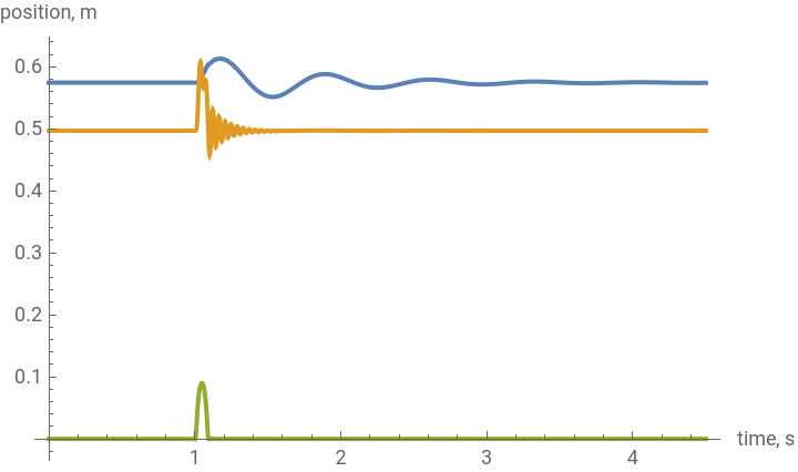
Plot positions:
In[]:=
Plot[Evaluate[{x[t],y[t],h[t]}/.sol],{t,0,timeStop},PlotLegends->{"x1(t)","x2(t)"},AxesLabel->{"time, s","position, m"},PlotRange->All]
Out[]=


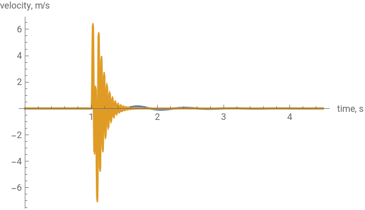
Plot velocities:
In[]:=
Plot[Evaluate[{vx[t],vy[t]}/.sol],{t,0,timeStop},PlotLegends->{"velocity of x1(t)","velocity of x2(t)"},AxesLabel->{"time, s","velocity, m/s"},PlotRange->All]
Out[]=
Plot accelerations:
In[]:=
Plot[Evaluate[{ax[t],ay[t]}/.sol],{t,0,timeStop},PlotLegends->{"acceleration of x1(t)","acceleration of x2(t)"},AxesLabel->{"time, s","acceleration, m/"},PlotRange->All]
2
s
Out[]=
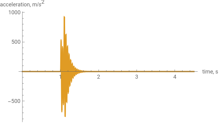
As you see, accelerations do indeed acquire large values. I think this is just the nature of the simplified description of the problem, with limited space for things like additional deformation effects that would manifest in real life as well as the possibility for the bike to simply rise above the ground.
If you are interested in or familiar with the system modeling functionality, you can verify this with the System Modeler tool, that allows you to easily model these systems with drag and dropping components and their connections. A simple version of the model can be loaded here:
In[]:=
model=ImportString,"MO";
See the diagram:
In[]:=
SystemModel[model,"Diagram"]
Out[]=
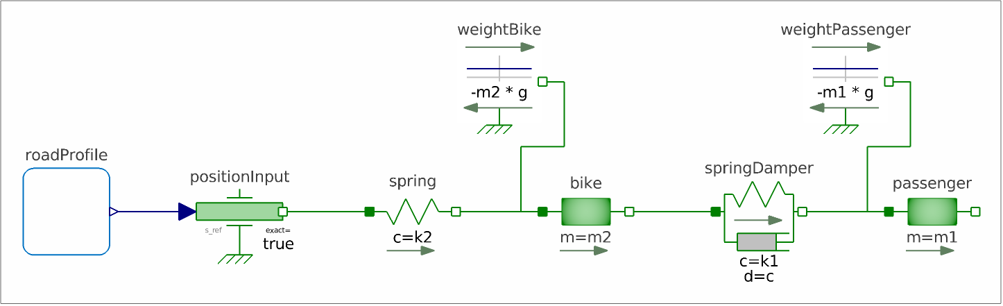
Use the SystemModelManipulate resource function to simulate and plot the model while manipulating the values of parameters in the model: (to simulate you may need to set a compiler in your configuration)
In[]:=
Out[]=