Define a list of RGB colors for blending in plots
In[]:=
clrs={,,,,,,,,,,,,,,,,,,,,,,};

Set parameters for the number of terms in the model
kM=50;nM=50;
Initialize the random number generator with a fixed seed for reproducibility
SeedRandom[23];
Generate random real numbers for p1 and p2 with a uniform distribution between -1 and 1
{p1,p2}=RandomReal[10{-1,1},{2,nM,kM}];
Generate random integer choices for q1 and q2 from the set {-2, -1, 1, 2}
{q1,q2}=RandomChoice[{-2,-1,1,2},{2,nM,kM}];
Define a complex function g[t][z] that that evolves over time and varies with the complex variable z
g[t_][z_]=TotalTable,{n,nM};
Product[z+p1[[n,k]]Exp[q1[[n,k]]It],{k,kM}]
Product[z+p2[[n,k]]Exp[q2[[n,k]]It],{k,kM}]
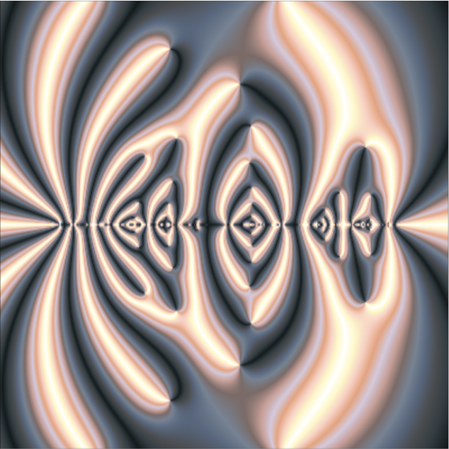
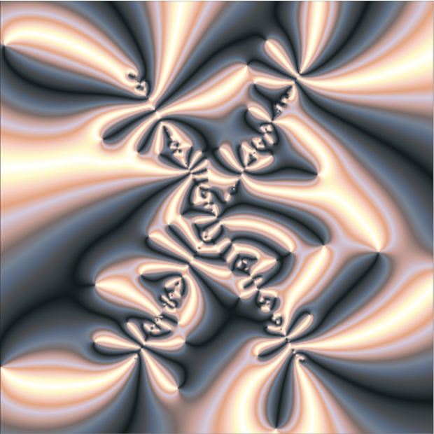
The function g[t][z] is a dynamic complex function that evolves over time t and depends on the complex variable z. Mathematically, it is defined as the sum of nM terms, where each term is the ratio of two products, each containing kM factors. Specifically, for each n from 1 to nM, the numerator is the product of expressions (z + p1[[n, k]] * Exp[q1[[n, k]] * I * t]) for k from 1 to kM, and the denominator is the product of (z + p2[[n, k]] * Exp[q2[[n, k]] * I * t]) for the same range of k. Here, p1 and p2 are arrays of randomly generated real numbers, while q1 and q2 contain randomly chosen integers from the set {-2, -1, 1, 2}. The exponential terms introduce time-dependent oscillations, causing each factor to rotate in the complex plane as t changes. This results in a highly intricate and time-varying function whose behavior is influenced by the interplay of multiple randomly assigned coefficients. When visualized using ComplexPlot and animated over time, g[t][z] generates rich and evolving patterns in the complex plane, with colors blended from the predefined clrs palette to highlight different regions and magnitudes. The combination of high-degree polynomials and dynamic oscillations creates mesmerizing visuals that illustrate the complex interactions and transformations within the function as time progresses.
Plot the complex function g at time t = 0
In[]:=
ComplexPlot[g[0][z],{z,13(-1-I),13(1+I)},ColorFunction->{Blend[clrs,#8]&,None},ImageSize->1000,PerformanceGoal->"Speed",Frame->False,PlotRangePadding->None]
Out[]=
Plot the complex function g at time t = Pi/3
In[]:=
ComplexPlot[g[Pi/3][z],{z,13(-1-I),13(1+I)},ColorFunction->{Blend[clrs,#8]&,None},ImageSize->1000,PerformanceGoal->"Speed",Frame->False,PlotRangePadding->None]
Out[]=
Create an animation video of the complex function g over time from 0 to 2 Pi
Parallelize@AnimationVideo[ComplexPlot[g[t][z],{z,13(-1-I),13(1+I)},ColorFunction->{Blend[clrs,#8]&,None},ImageSize->1080,PerformanceGoal->"Quality",Frame->False,PlotRangePadding->None],{t,0,2Pi},RasterSize->1080,DefaultDuration->20];//AbsoluteTiming
Out[]=
CITE THIS NOTEBOOK
CITE THIS NOTEBOOK
Infinities and zeros of functions on the complex plane with randomized structure
by Vitaliy Kaurov
Wolfram Community, STAFF PICKS, January 14, 2025
https://community.wolfram.com/groups/-/m/t/3356562
by Vitaliy Kaurov
Wolfram Community, STAFF PICKS, January 14, 2025
https://community.wolfram.com/groups/-/m/t/3356562