ABSTRACT (original article): The Effective Field Theory of Large Scale Structure (EFTofLSS) has found tremendous success as a perturbative framework for the evolution of large scale structure, and it is now routinely used to compare theoretical predictions against cosmological observations. The model for the total matter field includes one nuisance parameter at 1-loop order, the effective sound speed, which can be extracted by matching the EFT to full N-body simulations. In this work we first leverage the Layzer-Irvine cosmic energy equation to show that the equation of state can be exactly computed with knowledge of the fully nonlinear power spectrum. When augmented with separate universe methods, we show one can estimate the effective sound speed. This estimate is in good agreement with simulation results, with errors at the few tens of percent level. We apply our method to investigate the cosmology dependence of the effective sound speed and to shed light on what cosmic structures shape its value. CITATION (original article): Caio Nascimento, Drew Jamieson, Matthew McQuinn, Marilena Loverde (2024), arXiv:2410.11949. https://doi.org/10.48550/arXiv.2410.11949
This notebook computes an estimate for the effective sound speed as a function of the smoothing scale. The effective sound speed is a key free parameter introduced in the effective field theory of large scale structure, a theory introduced to model the effects of nonlinear gravitational evolution in the distribution of matter in our Universe.
In[]:=
Needs["MaTeX`"]
Introduce relevant parameters
In[]:=
h:=0.688H0:=omegamt:=0.295omegalt:=1-omegamt
100*h
299792
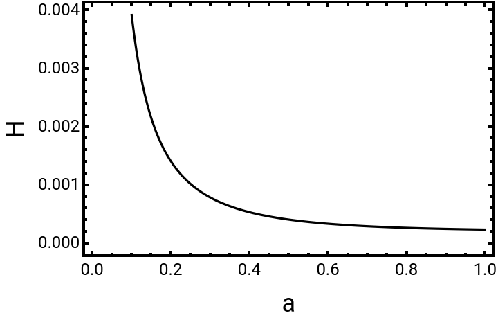
Compute hubble expansion rate
In[]:=
H[a_]:=H0*
omegamt*+omegalt
-3
a
In[]:=
Plot[H[a],{a,0,1},FrameStyleDirective[Thick,Black,12],FrameTrue,FrameLabel{Style["a",Black,18],Style["H",Black,18]},PlotStyleBlack]
Out[]=
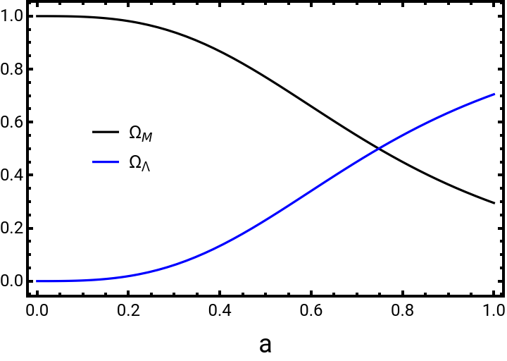
Compute fractional contributions to energy density, from matter and dark energy
In[]:=
omegam[a_]:=omegal[a_]:=
omegamt*
-3
a
omegamt*+omegalt
-3
a
omegalt
omegamt*+omegalt
-3
a
In[]:=
Plot[{omegam[a],omegal[a]},{a,0,1},FrameStyleDirective[Thick,Black,12],FrameTrue,FrameLabel{Style["a",Black,18],None},PlotStyle{Black,Blue},PlotLegendsPlaced[{"",""},{{0.2,0.5}}],PlotRangeAll]
Ω
M
Ω
Λ
Out[]=
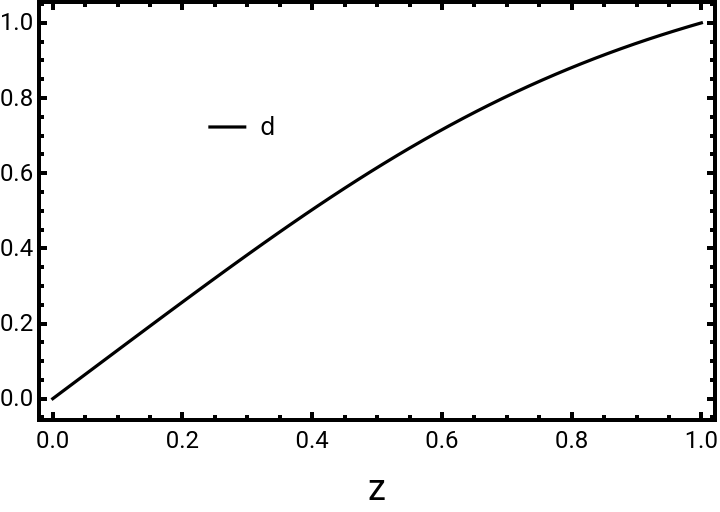
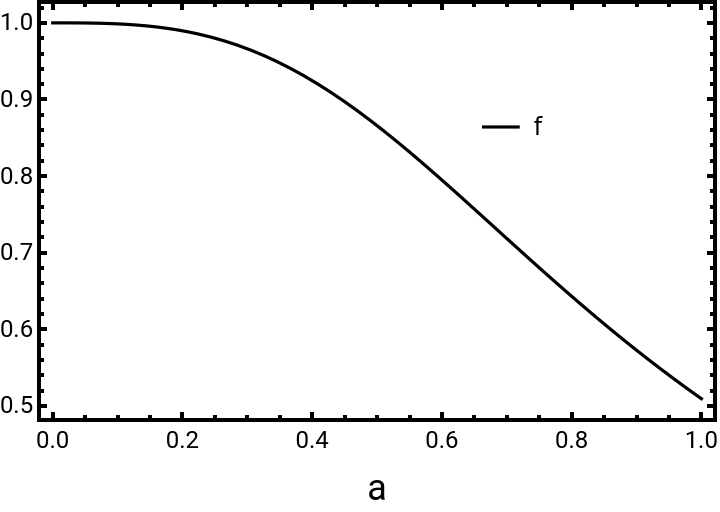
Compute (approximate) linear growth factor and rate
In[]:=
dt:=
5*omegam[1]
2*-omegal[1]+1+*1+
4
7
omegam[1]
omegam[1]
2
omegal[1]
70
In[]:=
d[a_]:=*
1
dt
5*omegam[a]*a
2*-omegal[a]+1+*1+
4
7
omegam[a]
omegam[a]
2
omegal[a]
70
In[]:=
Plot[d[a],{a,0,1},FrameStyleDirective[Thick,Black,12],FrameTrue,FrameLabel{Style["z",Black,18],None},PlotStyle{Black},PlotLegendsPlaced[{"d"},{{0.3,0.7}}],PlotRangeAll]
Out[]=
In[]:=
f[a_]:=+1+*
4
7
omegam[a]
omegam[a]
2
omegal[a]
70
In[]:=
Plot[f[a],{a,0,1},FrameStyleDirective[Thick,Black,12],FrameTrue,FrameLabel{Style["a",Black,18],None},PlotStyle{Black},PlotLegendsPlaced[{"f"},{{0.7,0.7}}],PlotRangeAll]
Out[]=
Import matter power spectrum
In[]:=
mpsl=Import["C:\\Users\\caios\\OneDrive\\Documents\\Matching_EFTofLSS\\Data\\mpsl.mx"]
Out[]=
InterpolatingFunction


In[]:=
mps=Import["C:\\Users\\caios\\OneDrive\\Documents\\Matching_EFTofLSS\\Data\\mps.mx"]
Out[]=
InterpolatingFunction

In[]:=
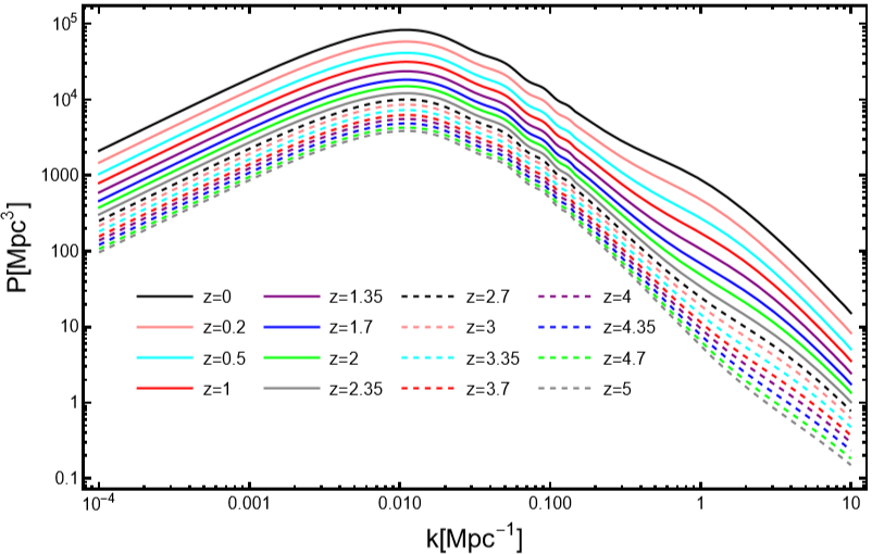
LogLogPlotmps,k,mps,k,mps,k,mps,k,mps,k,mps,k,mps,k,mps,k,mps,k,mps,k,mps,k,mps,k,mps,k,mps,k,mps,k,mps,k,{k,,10},FrameStyleDirective[Thick,Black,12],FrameTrue,FrameLabel{Style["k[]",Black,18],Style["P[]",Black,18]},PlotStyle{Black,Pink,Cyan,Red,Purple,Blue,Green,Gray,Directive[Dashed,Black],Directive[Dashed,Pink],Directive[Dashed,Cyan],Directive[Dashed,Red],Directive[Dashed,Purple],Directive[Dashed,Blue],Directive[Dashed,Green],Directive[Dashed,Gray]},PlotRangeAll,PlotLegendsPlaced[{"z=0","z=0.2","z=0.5","z=1","z=1.35","z=1.7","z=2","z=2.35","z=2.7","z=3","z=3.35","z=3.7","z=4","z=4.35","z=4.7","z=5"},{{0.4,0.3}}]
1
1+0
1
1+0.35
1
1+0.7
1
1+1
1
1+1.35
1
1+1.7
1
1+2
1
1+2.35
1
1+2.7
1
1+3
1
1+3.35
1
1+3.7
1
1+4
1
1+4.35
1
1+4.7
1
1+5
-4
10
-1
Mpc
3
Mpc
Out[]=
In[]:=
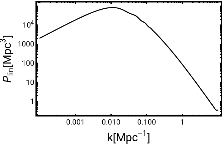
LogLogPlotmpsl[k],{k,,10},FrameStyleDirective[Thick,Black,12],FrameTrue,FrameLabelStyle["k[]",Black,18],Style"[]",Black,18,PlotStyleBlack,PlotRangeAll
-4
10
-1
Mpc
P
lin
3
Mpc
Out[]=
Import relevant halo model quantities
Compute halo model response function
Compute equation of state, including both potential and kinetic contributions
Take derivatives of the equation of state with respect to a long-wavelength mode
Compute the equation of state
Compute the renormalized effective sound speed from simulations
Use the RG flow to run the simulation result to finite cutoff scale
Compare analytically estimated and simulation results
CITE THIS NOTEBOOK
CITE THIS NOTEBOOK
A semi-analytic estimate for the effective sound speed counterterm in the EFTofLSS
by Caio Nascimento, Drew Jamieson, Matthew McQuinn & Marilena Loverde
Wolfram Community, STAFF PICKS, November 1, 2024
https://community.wolfram.com/groups/-/m/t/3313236
by Caio Nascimento, Drew Jamieson, Matthew McQuinn & Marilena Loverde
Wolfram Community, STAFF PICKS, November 1, 2024
https://community.wolfram.com/groups/-/m/t/3313236