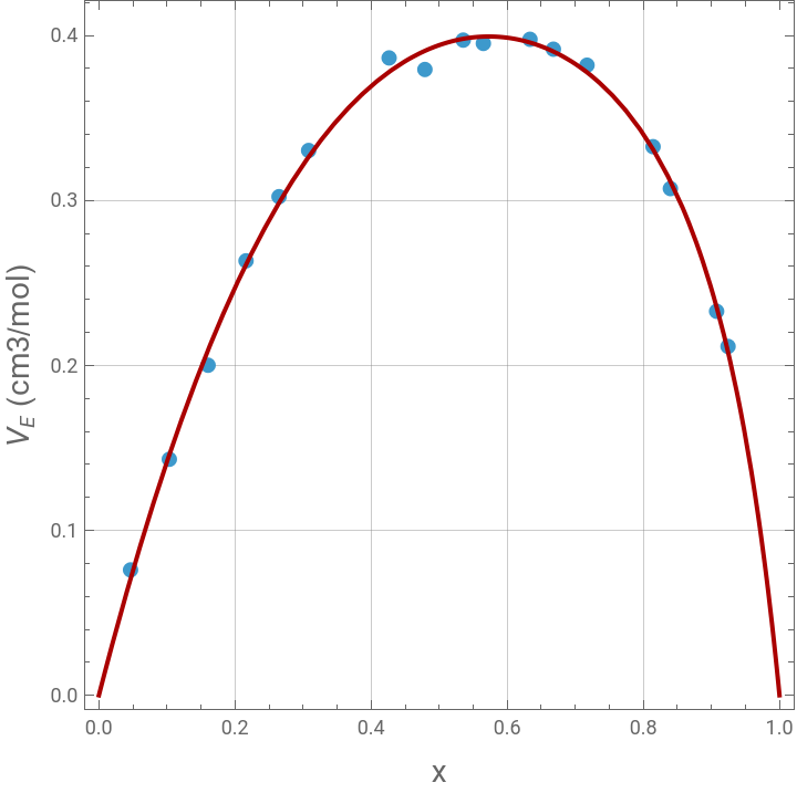
The excess molar volume behavior of the ethanol–hexane system at 298.15 K was investigated by Jiménez et al. (2000) through density measurements over the entire composition range. The authors found that the excess molar volume () is positive for all mixture compositions, indicating volume expansion upon mixing. A maximum positive deviation occurs at intermediate ethanol mole fractions.
This positive excess volume is attributed primarily to the disruption of the hydrogen-bonded structure of pure ethanol when hexane molecules are introduced. The breaking of ethanol–ethanol hydrogen bonds reduces molecular packing efficiency and creates additional free volume within the liquid mixture. Since the interactions between ethanol and the nonpolar hexane molecules are weaker than the original hydrogen-bond interactions, the structural expansion is not compensated by attractive intermolecular forces, resulting in volume dilatation. Therefore, the positive () values reflect the predominance of hydrogen-bond breakage and the inefficient packing between polar ethanol and nonpolar hexane molecules.
V
E
This positive excess volume is attributed primarily to the disruption of the hydrogen-bonded structure of pure ethanol when hexane molecules are introduced. The breaking of ethanol–ethanol hydrogen bonds reduces molecular packing efficiency and creates additional free volume within the liquid mixture. Since the interactions between ethanol and the nonpolar hexane molecules are weaker than the original hydrogen-bond interactions, the structural expansion is not compensated by attractive intermolecular forces, resulting in volume dilatation. Therefore, the positive (
V
E
The Redlich–Kister equation is commonly used to correlate excess properties of binary mixtures such as excess molar volume, excess Gibbs energy, refractive index deviations, and surface tension deviations.
The Redlich–Kister parameters reported in Table 5 were recalculated using Mathematica based on the experimental data for the ethanol–hexane system at 298.15 K. The computed coefficients for excess molar volume, surface tension, and refractive index were found to be in excellent agreement with the literature values. Furthermore, the standard deviations obtained from the regressions closely matched those reported by the authors, confirming the accuracy and reliability of the numerical implementation. This agreement demonstrates that the Mathematica procedure successfully reproduces the correlations and statistical quality of the original work.
The Redlich–Kister parameters reported in Table 5 were recalculated using Mathematica based on the experimental data for the ethanol–hexane system at 298.15 K. The computed coefficients for excess molar volume, surface tension, and refractive index were found to be in excellent agreement with the literature values. Furthermore, the standard deviations obtained from the regressions closely matched those reported by the authors, confirming the accuracy and reliability of the numerical implementation. This agreement demonstrates that the Mathematica procedure successfully reproduces the correlations and statistical quality of the original work.
Excess Molar Volume of Hexane + Ethanol Mixture at 298.15 K
Excess Molar Volume of Hexane + Ethanol Mixture at 298.15 K
In[]:=
data={{0.0465,0.076},{0.1035,0.1431},{0.1604,0.2001},{0.2162,0.2634},{0.2647,0.3023},{0.3082,0.3303},{0.4264,0.3864},{0.479,0.3794},{0.5353,0.3972},{0.5649,0.3952},{0.6334,0.3977},{0.6678,0.3917},{0.7172,0.382},{0.8142,0.3326},{0.8397,0.3072},{0.9076,0.2328},{0.9244,0.2115}};
In[]:=
p1=ListPlot[data,AspectRatio->1,GridLines->Automatic,Frame->True,PlotStyle->Thick,PlotMarkers->Automatic];
In[]:=
nlm1=NonlinearModelFit[data,x(1-x)/(1+B0(2x-1))Sum[A[k](2x-1)^k,{k,0,2}],{A[0],A[1],A[2],B0},x];
In[]:=
Normal[nlm1]
Out[]=
(1-x)x(1.57668-0.911456(-1+2x)+0.349957)
2
(-1+2x)
1-0.760659(-1+2x)
In[]:=
nlm1[{"ParameterTable","RSquared"}]
Out[]=
,0.999744
Estimate | Standard Error | t-Statistic | P-Value | |
A[0] | 1.57668 | 0.0104951 | 150.23 | 1.89632× -22 10 |
A[1] | -0.911456 | 0.107492 | -8.4793 | 1.17595× -6 10 |
A[2] | 0.349957 | 0.0743268 | 4.70835 | 0.000409004 |
B0 | -0.760659 | 0.0575731 | -13.2121 | 6.53621× -9 10 |
Variance
nlm1["EstimatedVariance"]
Out[]=
0.0000336039
Standard deviation
Sqrt[%]
Out[]=
0.00579689
p-values indicate that we should not retain nlm2
In[]:=
nlm2=NonlinearModelFit[data,x(1-x)/(1+B0(2x-1))Sum[A[k](2x-1)^k,{k,0,3}],{A[0],A[1],A[2],A[3],B0},x];
In[]:=
Normal[nlm2]
Out[]=
(1-x)x(1.57673-0.832734(-1+2x)+0.381426+0.0923089)
2
(-1+2x)
3
(-1+2x)
1-0.701125(-1+2x)
In[]:=
nlm2[{"ParameterTable","RSquared"}]
Out[]=
,0.999746
Estimate | Standard Error | t-Statistic | P-Value | |
A[0] | 1.57673 | 0.0109956 | 143.397 | 8.88177× -21 10 |
A[1] | -0.832734 | 0.235848 | -3.53081 | 0.00414026 |
A[2] | 0.381426 | 0.112728 | 3.38358 | 0.00543207 |
A[3] | 0.0923089 | 0.243254 | 0.379476 | 0.710965 |
B0 | -0.701125 | 0.167217 | -4.19291 | 0.00124753 |
In[]:=
p2=Plot[Normal[nlm1],{x,0,1},AspectRatio->1,GridLines->Automatic,Frame->True,PlotStyle->{Darker@Red,Thick}];
In[]:=
Show[p1,p2,PlotRange->{{0,1},Automatic},FrameLabel->{Style["x",14],Style[" (cm3/mol)",14]}]
V
E
Out[]=
Surface Tension of Hexane + Ethanol Mixture at 298.15 K
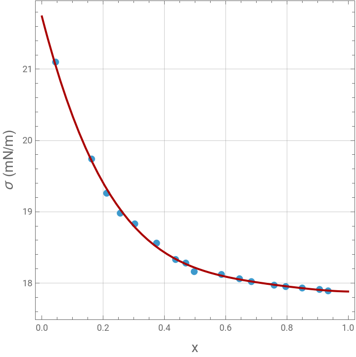
Surface Tension of Hexane + Ethanol Mixture at 298.15 K
In[]:=
data={{0.0448,21.1},{0.1625,19.74},{0.2116,19.26},{0.2559,18.98},{0.3034,18.83},{0.3745,18.56},{0.4366,18.33},{0.47,18.28},{0.4974,18.16},{0.5863,18.12},{0.6452,18.06},{0.6841,18.02},{0.7584,17.97},{0.7963,17.95},{0.85,17.93},{0.9067,17.91},{0.9347,17.89}};
In[]:=
p1=ListPlot[data,AspectRatio->1,GridLines->Automatic,Frame->True,PlotStyle->Thick,PlotMarkers->Automatic];
In[]:=
nlm1=NonlinearModelFit[data,21.74+Sum[A[k]x^(k+1),{k,0,3}],{A[0],A[1],A[2],A[3]},x];
In[]:=
Normal[nlm1]
Out[]=
21.74-16.6411x+29.3764-24.1992+7.60474
2
x
3
x
4
x
Variance
nlm1["EstimatedVariance"]
Out[]=
0.00142704
Standard deviation
Sqrt@%
Out[]=
0.0377761
In[]:=
nlm1[{"ParameterTable","RSquared"}]
Out[]=
,0.999997
Estimate | Standard Error | t-Statistic | P-Value | |
A[0] | -16.6411 | 0.364157 | -45.6977 | 9.6001× -16 10 |
A[1] | 29.3764 | 2.02157 | 14.5315 | 2.04069× -9 10 |
A[2] | -24.1992 | 3.49915 | -6.91573 | 0.0000105984 |
A[3] | 7.60474 | 1.90126 | 3.99984 | 0.00151254 |
p-values indicate that we should not retain nlm2
In[]:=
nlm2=NonlinearModelFit[data,21.74+Sum[A[k]x^(k+1),{k,0,4}],{A[0],A[1],A[2],A[3],A[4]},x];
In[]:=
Normal[nlm2]
Out[]=
21.74-16.429x+27.4367-18.343+0.442263+3.06289
2
x
3
x
4
x
5
x
In[]:=
nlm2[{"ParameterTable","RSquared"}]
Out[]=
,0.999997
Estimate | Standard Error | t-Statistic | P-Value | |
A[0] | -16.429 | 0.750066 | -21.9034 | 4.81364× -11 10 |
A[1] | 27.4367 | 6.28692 | 4.3641 | 0.000921701 |
A[2] | -18.343 | 18.2606 | -1.00451 | 0.334957 |
A[3] | 0.442263 | 21.9774 | 0.0201235 | 0.984276 |
A[4] | 3.06289 | 9.36034 | 0.32722 | 0.749139 |
In[]:=
p2=Plot[Normal[nlm1],{x,0,1},AspectRatio->1,GridLines->Automatic,Frame->True,PlotStyle->{Darker@Red,Thick}];
In[]:=
Show[p1,p2,PlotRange->{{0,1},All},FrameLabel->{Style["x",14],Style["σ (mN/m)",14]}]
Out[]=
Refractive Index of Hexane + Ethanol Mixture at 298.15 K
Refractive Index of Hexane + Ethanol Mixture at 298.15 K
In[]:=
data={{0.1604,1.3619},{0.2162,1.3627},{0.3745,1.3649},{0.4366,1.3657},{0.5353,1.3669},{0.5863,1.3674},{0.6334,1.3679},{0.6452,1.3681},{0.6678,1.3684},{0.7172,1.3689},{0.7584,1.3694},{0.7963,1.3698},{0.8397,1.3703},{0.9067,1.3711}};
In[]:=
p1=ListPlot[data,AspectRatio->1,GridLines->Automatic,Frame->True,PlotStyle->Thick,PlotMarkers->Automatic];
In[]:=
nlm1=NonlinearModelFit[data,1.3593+Sum[A[k]x^(k+1),{k,0,2}],{A[0],A[1],A[2]},x];
In[]:=
Normal[nlm1]
Out[]=
1.3593+0.017622x-0.00876782+0.00404129
2
x
3
x
Variance
nlm1["EstimatedVariance"]
Out[]=
1.48505×
-9
10
Standard deviation
Sqrt@%
Out[]=
0.0000385363
In[]:=
nlm1[{"ParameterTable","RSquared"}]
Out[]=
,1.
Estimate | Standard Error | t-Statistic | P-Value | |
A[0] | 0.017622 | 0.000220048 | 80.0825 | 1.43335× -16 10 |
A[1] | -0.00876782 | 0.000677634 | -12.9389 | 5.3435× -8 10 |
A[2] | 0.00404129 | 0.000513808 | 7.86537 | 7.67332× -6 10 |
p-values indicate that we should not retain nlm2
In[]:=
nlm2=NonlinearModelFit[data,1.3593+Sum[A[k]x^(k+1),{k,0,3}],{A[0],A[1],A[2],A[3]},x];
In[]:=
Normal[nlm2]
Out[]=
1.3593+0.0170105x-0.0050348-0.00269936+0.00375097
2
x
3
x
4
x
In[]:=
nlm2[{"ParameterTable","RSquared"}]
Out[]=
,1.
Estimate | Standard Error | t-Statistic | P-Value | |
A[0] | 0.0170105 | 0.000430621 | 39.5023 | 2.58323× -12 10 |
A[1] | -0.0050348 | 0.00239523 | -2.10201 | 0.0618679 |
A[2] | -0.00269936 | 0.00419884 | -0.642882 | 0.534763 |
A[3] | 0.00375097 | 0.00232122 | 1.61595 | 0.137178 |
References
References
[1] Eulogio Jiménez, Herminio Casas, Luisa Segade, and Carlos Franjo, Surface Tensions, Refractive Indexes and Excess Molar Volumes of Hexane + 1-Alkanol Mixtures at 298.15 K, Journal of Chemical & Engineering Data, 45, 2000, pp. 862-866. DOI: 10.1021/je000060k
CITE THIS NOTEBOOK
CITE THIS NOTEBOOK
Surface tension, refractive index, & excess molar volume of hexane+ethanol mixture at 298.15 K
by Housam Binous
Wolfram Community, STAFF PICKS, June 4, 2026
https://community.wolfram.com/groups/-/m/t/3727150
by Housam Binous
Wolfram Community, STAFF PICKS, June 4, 2026
https://community.wolfram.com/groups/-/m/t/3727150