ABSTRACT (original article): Hash Chemistry, a minimalistic artificial chemistry model of open-ended evolution, has recently been extended to non-spatial and cellular versions. The non-spatial version successfully demonstrated continuous adaptation and unbounded growth of complexity of self-replicating entities, but it did not simulate multiscale ecological interactions among the entities. On the contrary, the cellular version explicitly represented multiscale spatial ecological interactions among evolving patterns, yet it failed to show meaningful adaptive evolution or complexity growth. It remains an open question whether it is possible to create a similar minimalistic evolutionary system that can exhibit all of those desired properties at once within a computationally efficient framework. Here we propose an improved version called Structural Cellular Hash Chemistry (SCHC). In SCHC, individual identities of evolving patterns are explicitly represented and processed as the connected components of the nearest neighbor graph of active cells. The neighborhood connections are established by connecting active cells with other active cells in their Moore neighborhoods in a 2D cellular grid. Evolutionary dynamics in SCHC are simulated via pairwise competitions of two randomly selected patterns, following the approach used in the non-spatial Hash Chemistry. SCHC’s computational cost was significantly less than the original and non-spatial versions. Numerical simulations showed that these model modifications achieved spontaneous movement, self-replication and unbounded growth of complexity of spatial evolving patterns, which were clearly visible in space in a highly intuitive manner. Detailed analysis of simulation results showed that there were spatial ecological interactions among self-replicating patterns and their diversity was also substantially promoted in SCHC, neither of which was present in the non-spatial version. CITATION (original article): Hiroki Sayama (2024), Structural Cellular Hash Chemistry, arXiv:2412.12790. https://doi.org/10.48550/arXiv.2412.12790
GitHub: https://github.com/hsayama/Structural-Cellular-Hash-Chemistry
GitHub: https://github.com/hsayama/Structural-Cellular-Hash-Chemistry
Warning: Sections 3 and 4 involve intensive computations and generate files that will be saved to the local hard disk. Please run them with care.
1. Definitions
1. Definitions
2. Interactive Demo
2. Interactive Demo
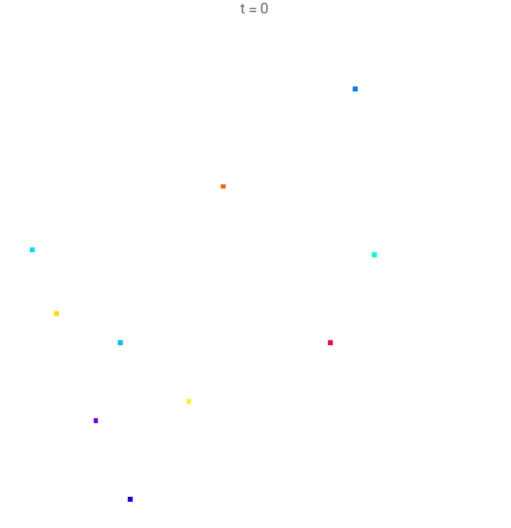
Here is a visual demo of the simulation run of Structural Cellular Hash Chemistry. Colors represent different element types, and blank (white) spaces represent empty cells. It is observed in these visualizations that the self-replicating patterns gradually proliferate and evolved to larger forms with more complex nontrivial structures.
The function that simulates one update step in the system. It selects two connected components randomly, calculates their fitness, and makes them compete. The winner’s pattern is copied over the loser’s position in the grid, with mutations applied.
update
In[]:=
update[config_]:=Module[{numActiveCells,nng,c1,c2,r1,r2,p1,p2,x,f1,f2,winner},numActiveCells=Length[activeCells];If[numActiveCells==0,Return[config]];c1=connectedComponentCells[config,RandomChoice[activeCells]];c2=connectedComponentCells[config,RandomChoice[activeCells]];r1=Transpose[MinMax/@(c1//Transpose)];r2=Transpose[MinMax/@(c2//Transpose)];p1=Table[{x-r1[[1]],config[[x[[1]],x[[2]]]]},{x,c1}]//Sort;p2=Table[{x-r2[[1]],config[[x[[1]],x[[2]]]]},{x,c2}]//Sort;{f1,f2}=fitness/@{p1,p2};winner=RandomChoice[Position[#,Max[#]]&[{f1,f2}]//Flatten];winnerproportion=N[Length[{c1,c2}[[winner]]]/numActiveCells];Switch[winner,1,Return[rewrite[config,r1,r2]],2,Return[rewrite[config,r2,r1]]];];
In[]:=
config=Table[None,L,L];activeCells={};Do[While[True,{x,y}=RandomInteger[{1,L},2];If[config[[x,y]]==None,Break[]]];config[[x,y]]=RandomInteger[{1,k}];AppendTo[activeCells,{x,y}];,n];time=0;onestep[]:=Module[{elapsed=0.},While[elapsed<1.,config=update[config];elapsed=elapsed+winnerproportion;winnerproportion=0.;];];Manipulate[If[run,ClearSystemCache[];onestep[];time+=1;];plot[config,time],{{run,False},{True,False}},TrackedSymbols{run,config,time},SaveDefinitions->True]
Out[]=

3. Systematic Simulations
3. Systematic Simulations
The code sets up a simulation environment for running 100 independent trials of the SCHC model. Each trial runs for 2000 iterations, and the resulting data is logged to files. The simulation uses the previously defined update mechanism to evolve the grid over time.
updateSim[config_]:=Module[{numActiveCells,nng,c1,c2,r1,r2,p1,p2,x,f1,f2,winner},numActiveCells=Length[activeCells];If[numActiveCells==0,Return[config]];c1=connectedComponentCells[config,RandomChoice[activeCells]];c2=connectedComponentCells[config,RandomChoice[activeCells]];r1=Transpose[MinMax/@(c1//Transpose)];r2=Transpose[MinMax/@(c2//Transpose)];p1=Table[{x-r1[[1]],config[[x[[1]],x[[2]]]]},{x,c1}]//Sort;p2=Table[{x-r2[[1]],config[[x[[1]],x[[2]]]]},{x,c2}]//Sort;{f1,f2}=fitness/@{p1,p2};winner=RandomChoice[Position[#,Max[#]]&[{f1,f2}]//Flatten];winnerproportion=N[Length[{c1,c2}[[winner]]]/numActiveCells];Write[file,{time,{p1,p2}[[winner]],{f1,f2}[[winner]]}];Switch[winner,1,Return[rewrite[config,r1,r2]],2,Return[rewrite[config,r2,r1]]];];
In[]:=
SetDirectory[NotebookDirectory[]];
Monitor[Do[config=Table[None,L,L];activeCells={};Do[While[True,{x,y}=RandomInteger[{1,L},2];If[config[[x,y]]==None,Break[]]];config[[x,y]]=RandomInteger[{1,k}];AppendTo[activeCells,{x,y}];,n];time=0;onestep[]:=Module[{elapsed=0.},While[elapsed<1.,config=updateSim[config];elapsed=elapsed+winnerproportion;winnerproportion=0.;];];file=OpenWrite["fhistory-final-"<>ToString[ii]<>".dat"];While[time<2000,ClearSystemCache[];onestep[];time+=1;];Close[file];,{ii,100}],{ii,time}]
4. Plotting and Curve Fitting
4. Plotting and Curve Fitting
Importing aggregated data files
Importing aggregated data files
Formatting the data
Plotting
Plotting
The following plot is maximum fitness value observed in each time step. It showed a continuous increase over time.
Average fitness value in each time step. It showed an initial increase followed by a slight decrease in the long run.
The following are cumulative numbers of observed unique types that appeared in successful replication in the course of simulation. First a plot for cumulative number of observed cell types, then a plot for cumulative number of observed pattern (connected component) types. The red curves show results of 87 independent simulation runs, while the black solid curve shows their average. The time is again in log scale. Note that the curves in the top plot saturate at the maximal number of types (k = 1000), whereas the curves in the bottom plot grow toward substantially large numbers without bound.
Statistical model curve fitting
Statistical model curve fitting
This code creates a nonlinear model fit for the meancurve data using a bounded growth model. It returns a fitted model object, which contains the estimated parameters a and b along with other details about the fit.
Retrieving the best-fit expression from the bounded growth model created earlier
Extracting and returning various goodness-of-fit statistics for the bounded growth model, including the Akaike Information Criterion (AIC), Bayesian Information Criterion (BIC), R-squared, and adjusted R-squared values.
Performing a nonlinear model fit for meancurve using an unbounded growth model. The result is a fitted model object containing the estimated parameters a and b and additional fit information.
Retrieving the best-fit expression from the unbounded growth model created earlier
The code retrieves various fit statistics for the unbounded growth model, including the Akaike Information Criterion (AIC), Bayesian Information Criterion (BIC), R-squared, and adjusted R-squared values. These metrics help assess the model’s performance and compare it to other models.
The following are maximum and average numbers of active cells in replicating patterns. The red curves show results of 87 independent simulation runs, while the black solid curve shows their average. The time is in log scale to show long-term trends clearly. Purple (dashed) and blue (solid) curves are two different growth models (purple: bounded growth, blue: unbounded growth) fitted to the average behaviors during the time period 100–2000. In both plots, the unbounded growth model (blue curve) was a significantly better fit. See Table I for more details.
CITE THIS NOTEBOOK
CITE THIS NOTEBOOK
Structural cellular hash chemistry
by Hiroki Sayama
Wolfram Community, STAFF PICKS, September 30, 2025
https://community.wolfram.com/groups/-/m/t/3553183
by Hiroki Sayama
Wolfram Community, STAFF PICKS, September 30, 2025
https://community.wolfram.com/groups/-/m/t/3553183