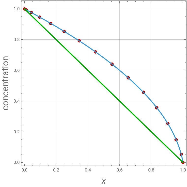
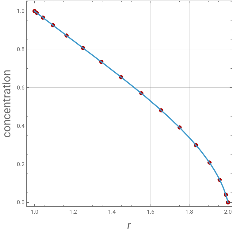
This notebook shows the steady-state concentration distribution through a plane sheet, a cylindrical annulus, and a spherical shell, in which diffusion is assumed to be one-dimensional.The relevant equations are:For the plane sheet, D=0 for , where is the diffusion coefficient and, without loss of generality, one can choose the boundary conditions and . Different values of parameter can be chosen. Here, we take α = 10.For the cylindrical annulus, Dr=0 for =1⩽r⩽=2, where is the diffusion coefficient. Again, one can choose the boundary conditions and . Again, we set α = 10.For the spherical shell, D=0 for =1⩽r⩽=2, with the same and boundary conditions as for the cylindrical annulus.For the plane sheet, if , then is a constant and the concentration distribution is indicated by the green line. Fick’s second law is recovered, as shown in the first plot.In all plots, the red dots correspond to the solution obtained using Chebyshev orthogonal collocation with collocation points (see Ref. 2). On the other hand, the blue curve is the implicit solution given by Crank [1]:For the plane sheet, .For the cylindrical annulus, .For the spherical shell, .For each of the three geometries, , , and .As expected, the two solutions agree perfectly.References:[1] J. Crank, The Mathematics of Diffusion, 2nd ed., New York: Oxford University Press, 1975.[2] Binous H., Kaddeche S., Bellagi A., Solution of six chemical engineering problems using the Chebyshev orthogonal collocation technique, Comput Appl Eng Educ., 2017; 25:594–607. https://doi.org/10.1002/cae.21823
∂
∂x
∂c
∂x
0⩽x⩽1
D=1+αc
c(x=0)=1
c(x=1)=0
α
1
r
∂
∂r
∂c
∂r
r
1
r
2
D=1+αc
c(r=1)=1
c(r=2)=0
1
2
r
∂
∂r
2
r
∂c
∂r
r
1
r
2
D
α=0
D=1
N=16
(A-c-F(c))/B=x
(A-c-F(c))/B=
ln()-ln(r)
r
1
ln()-ln()
r
1
r
2
(A-c-F(c))/B=(-r)
r
2
r
1
(-)r
r
1
r
2
A=1+F(1)
B=1+F(1)-0-F(0)
F(c)=αξdξ
c
∫
0
In[]:=
alpha=10;
In[]:=
Np=15;Ds=Table[d[i,j],{i,0,Np},{j,0,Np}];d[0,0]=(2Np^2+1)/6//N;d[Np,Np]=-(2Np^2+1)/6//N;d[i_,i_]:=-y[i]/(2(1-y[i]^2));y[i_]:=Cos[iPi/Np]//N;d[j_,k_]:=If[j≠k,c[j](-1)^(j+k)/(c[k](y[j]-y[k]))];
In[]:=
c[i_]:=If[i0||iNp,2,1];
In[]:=
r1=1;r2=2;
In[]:=
C1=1;C2=0;
Plane sheet case
In[]:=
x1=Table[1/2(y[i]+1),{i,Np,0,-1}];Concp[i_]:=Ds[[i,j]]conc[j];U1=Table[(1+alphaconc[j])Concp[j],{j,1,Np+1}];Eq[i_]:=Ds[[i]].U10;bc1=conc[1]1;bc2=conc[Np+1]0;initguess=Table[{conc[i],0.5},{i,1,Np+1}];sys=Flatten[{bc1,bc2,Table[Eq[i],{i,2,Np}]},1];sol=FindRoot[sys,initguess,MaxIterations1000];p1=ListPlot[Table[{x1[[i]],conc[i]/.sol},{i,1,Np+1}],FrameTrue,AspectRatio1,PlotStyle{Darker@Red,PointSize[0.02]}];F[Ci_?NumericQ]:=Quiet@NIntegrate[alphac,{c,0,Ci}];A=C1+F[C1];B=C1+F[C1]-C2-F[C2];p2=ContourPlot[(A-Cc-F[Cc])/Bx,{x,0,1},{Cc,0,1}];Show[p1,p2,Graphics[{Darker@Green,Thickness[0.007],Line[{{1,0},{0,1}}]}],ImageSize380{1,1},GridLinesAutomatic,FrameLabel{Style["x",Italic,18],Style["concentration",18]}]
Np+1
∑
j=1
Out[]=
Cylindrical annulus case
In[]:=
x1=Table[(r2-r1)/2(y[i]+1)+r1,{i,Np,0,-1}];F[Ci_?NumericQ]:=Quiet@NIntegrate[alphac,{c,0,Ci}];A=C1+F[C1];B=C1+F[C1]-C2-F[C2];p2=ContourPlot[(A-Cc-F[Cc])/B(Log[r1]-Log[r])/(Log[r1]-Log[r2]),{r,1,2},{Cc,0,1},PlotPoints10];Concp[i_]:=Ds[[i,j]]conc[j];U1=Table[x1[[j]](1+alphaconc[j])Concp[j],{j,1,Np+1}];Eq[i_]:=Ds[[i]].U10;bc1=conc[1]1;bc2=conc[Np+1]0;initguess=Table[{conc[i],0.5},{i,1,Np+1}];sys=Flatten[{bc1,bc2,Table[Eq[i],{i,2,Np}]},1];sol=FindRoot[sys,initguess,MaxIterations1000];p1=ListPlot[Table[{x1[[i]],conc[i]/.sol},{i,1,Np+1}],FrameTrue,AspectRatio1,PlotStyle{Darker@Red,PointSize[0.02]}];Show[p1,p2,ImageSize380{1,1},GridLinesAutomatic,FrameLabel{Style["r",Italic,18],Style["concentration",18]}]
Np+1
∑
j=1
Out[]=
Spherical shell case
In[]:=
x1=Table[(r2-r1)/2(y[i]+1)+r1,{i,Np,0,-1}];F[Ci_?NumericQ]:=Quiet@NIntegrate[alphac,{c,0,Ci}];A=C1+F[C1];B=C1+F[C1]-C2-F[C2];p2=ContourPlot[(A-Cc-F[Cc])/Br2/(r1-r2)(r1-r)/r,{r,1,2},{Cc,0,1},PlotPoints10];Concp[i_]:=Ds[[i,j]]conc[j];U1=Table[x1[[j]]^2(1+alphaconc[j])Concp[j],{j,1,Np+1}];Eq[i_]:=Ds[[i]].U10;bc1=conc[1]1;bc2=conc[Np+1]0;initguess=Table[{conc[i],0.5},{i,1,Np+1}];sys=Flatten[{bc1,bc2,Table[Eq[i],{i,2,Np}]},1];sol=FindRoot[sys,initguess,MaxIterations1000];p1=ListPlot[Table[{x1[[i]],conc[i]/.sol},{i,1,Np+1}],FrameTrue,AspectRatio1,PlotStyle{Darker@Red,PointSize[0.02]}];Show[p1,p2,ImageSize380{1,1},GridLinesAutomatic,FrameLabel{Style["r",Italic,18],Style["concentration",18]}]
Np+1
∑
j=1