I. Introduction
I. Introduction
In August of 2023, researchers at Fermilab released the most precise measurements of the muon magnetic anomaly, a measure of how different the measured gyromagnetic ratio is to the theoretical value of 2, at an uncertainty of 0.20 parts per million (ppm) (Aguillard et al. 2023, 5). This experiment is one of many pioneering physics beyond the Standard Model and asks theorists and experimentalists alike to question our methods predicting and measuring the behavior of elementary particles. Because the Muon g-2 project (also called E989) is such a groundbreaking experiment that required the most cutting-edge technology and leading minds in particle physics, it is not very approachable for most college students, despite its importance. This project seeks to summarize the experiment at an undergraduate physics level and simulate some of the muon behavior in Mathematica. The Muon g-2 experiment starts with a beam of protons launched against an Inconel target at a rate of about 12 collisions per second (Bottalico 2022, 6, 47). From this scattering, a certain number of pions are produced which then travel to the Muon Delivery Ring. There, they decay into muons that are sent to the g-2 storage ring where they experience a constant magnetic field of 1.45T (Fermilab 2020). As the muon orbits the storage ring, its magnetic moment undergoes precession, meaning the axis of its spin rotates about the direction of the external magnetic field. When the muon decays to neutrinos and electrons, the electrons fly off towards the direction of the magnetic moment and are detected while the neutrinos simply pass by. The energy and the population density of the electrons are recorded by the highly sensitive detectors lining the storage ring which allow the experimentalists to “see” how the magnetic moment precessed in the magnetic field. The Standard Model says that the g-factor (which comes from the gyromagnetic ratio of these precessions) should be 2, but experimental data has demonstrated deviations beyond the expected uncertainty. So because this g-factor is greater than the theoretical value, the Muon g-2 experiment has become a prime candidate for testing physics beyond the Standard Model.
Deriving Equations of Motion
Deriving Equations of Motion
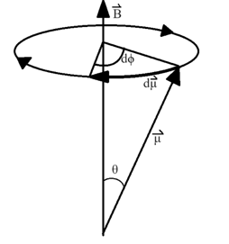
Fig 2. Precession of the muon’s moment in a magnetic field
The goal of this project was to model the muon g-2 experiment in Mathematica using equations of motion of spin precession, magnetic field simulation, and random variance. The first step was to understand the classical motion of how the magnetic moment of a muon would precess in a magnetic field. The time derivative of the magnetic moment vector of a particle (μ) is given by
μ
t
μ
B
where γ is the gyromagnetic ratio:
γ=*g
-e
2m
e here represents the charge of the particle, m is the mass, and g is the g-factor of interest. Classically, g=1 but the gyromagnetic ratio of a spinning muon/electron is different and Dirac’s equation gives g=2. Now assume that the magnetic field points in the z-direction with constant magnitude B (in an experiment setting, the coordinate system can be set to match this assumption). Then the cross product between the magnetic moment vector and the magnetic field gives us:
Derivations
In[]:=
Clear[B];Clear[Bfield];Bfield={0,0,B};μ[t_]:={μx[t],μy[t],μz[t]};
In[]:=
Clear[γ];dμ=γ*Cross[μ[t],Bfield]
Out[]=
{Bγμy[t],-Bγμx[t],0}
μ
x
t
Bγμ
y
μ
y
t
Bγμ
x
μ
z
t
Taking the time derivative again,
Derivations
In[]:=
d2μ=D[#,t]&/@dμ
Out[]=
{Bγ[t],-Bγ[t],0}
′
μy
′
μx
In[]:=
newd2μ=Replace[#,{[t]->dμ[[1]],[t]->dμ[[2]],[t]->dμ[[3]]},{1}]&/@d2μ//Simplify
′
μx
′
μy
′
μz
Out[]=
-μx[t],-μy[t],0
2
B
2
γ
2
B
2
γ
2
μ
x
2
t
2
B
2
γ
μ
x
2
μ
y
2
t
2
B
2
γ
μ
y
2
μ
z
2
t
The general solution to the second order differential equation for the x and y-components is a linear combination of the trigonometric functions:
μ
x
μ
y
First, the γB is angular velocity at which the magnetic moment vector precesses which is called the Larmor precession . And the first derivative of the x and y-components are each other, by using initial conditions:
ω
L
μ
z
μ
x
ω
L
μ
y
ω
L
μ
y
μ
y
ω
L
μ
x
ω
L
μ
z
μ
z
Since both the first and second derivative of the z-component are zero, it stays constant. When the muons are shot into the Storage Ring, they’re polarized in such a way that their spin and their momentum are colinear.If the gyromagnetic ratio was exactly 2, the momentum and spin vectors should remain colinear the entire way but in reality the spin vector starts to turn inwards towards the center of the ring (Fig. 3) (Bottalico 2022, 14). To reflect this, the initial position of the muon will be set along the positive y-axis and the moment vector will point straight in the x-direction.
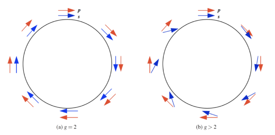
Fig 3. (a) Momentum vector for the muon (red) relative to its spin vector (blue) if g=2
(b) Momentum vector for the muon (red) relative to its spin vector (blue) if g>2
(b) Momentum vector for the muon (red) relative to its spin vector (blue) if g>2
Next, we can incorporate translational motion of this muon by applying Lorentz forces of a charged particle moving in a magnetic field. The magnetic field applies a torque that causes the muon to move in a circular path, so the equation of motion for position r(t) is:
m=q×
2
r
2
t
d
r
dt
B
By the same process as with magnetic moment, you get:
r
x
r
x
qB
m
r
y
qB
m
r
y
r
y
qB
m
r
x
qB
m
r
z
r
z
The angular frequency of this translational motion is the cyclotron frequency ).
(
ω
c
II. Animating Visuals
II. Animating Visuals
Defining Constraints for Classical Motion
In[]:=
g=2;(*g-factor*)γ=g*;(*gyromagneticratio*)B=1.45;(*magneticfield*)ωL=γ*B;(*Larmorprecessionfrequency*)
1.60217663*
-19
10
2(1.883531627*)
-28
10
In[]:=
ωC=(*cyclotronfrequency*)
(1.60217663*)(1.45)
-19
10
1.883531627*
-28
10
Out[]=
1.2334×
9
10
According to the National Institute of Standards and Technology, the magnetic moment of the muon has a magnitude of (NIST, n.d.)
4.49044830J·
-26
10
-1
T
In[]:=
μ0={4.4904483*,0,0};
-26
10
For the sake of visualization, muon storage ring will be taken to be very very small.
In[]:=
r0Fake={0,μ0[[1]]*10,0};
We will include the real radius for calculations and simulations later (Keshavarzi 2022, 4).
In[]:=
r0Real={0,7.112,0};
Equations of motion
Equations of motion
rX, rX, rX represent the spatial location of the muon and μX, μY, μZ represent the vector of the muon’s magnetic moment.
In[]:=
rX[t_]:=r0Fake[[1]]Cos[ωC*t]+r0Fake[[2]]Sin[ωC*t];rY[t_]:=r0Fake[[2]]Cos[ωC*t]-r0Fake[[1]]Sin[ωC*t];rZ[t_]:=r0Fake[[3]];μX[t_]:=μ0[[1]]Cos[ωL*t]+μ0[[2]]Sin[ωL*t];μY[t_]:=μ0[[2]]Cos[ωL*t]-μ0[[1]]Sin[ωL*t];μZ[t_]:=μ0[[3]];
The Muon Moment Vector
The Muon Moment Vector
The following animation is a visualization of the magnetic muon precessing due to an external magnetic field.
Code for animation
Combining with the Translational Path of the Muon
Combining with the Translational Path of the Muon
This will plot the path of the muon around the Storage Ring on which the muon (represented by the arrow of its spin) is superimposed on.
Code for animation
Observe how in this theoretical model, the momentum and spin vector are aligned as expected.
III. Adding Variance to the Magnetic Moment
III. Adding Variance to the Magnetic Moment
Randomly vary the Larmor precession frequency by changing the magnetic anomaly
New equations of motion
Code for animation
Code for animation
The red arrow represents the spin vector with the anomaly incorporated and the black arrow represents the classical model. As shown by the animation, the two arrows are closely aligned at the start but as time progresses, they start to point in different directions.
IV. Simulating the Magnetic Field
IV. Simulating the Magnetic Field
Fig 4. Coordinate axes of the Storage Ring
Initialize constants
Generating random coefficients for multipole contributions
Generate random Fourier expansion coefficients and phase shift angles
Calculates dipole moment contribution for the azimuthal slice at ϕ
V. Combining Nonuniform Magnetic Moment and Magnetic Field
V. Combining Nonuniform Magnetic Moment and Magnetic Field
Function to convert from Cartesian coordinates to r, θ, ϕ that the B-field function can recognize
Updated Larmor precession using nonuniform magnetic field
Muon travelling inside the Storage Ring (Realistic Scale)
Since this doesn’t provide any interesting information, the scale of the visualization can be modified.
Download the attached notebook for a running animation.
The black arrow represents the spin vector in classical motion, the red arrow represents the spin with the anomalous moment, and the blue arrow represents the spin with the anomalous moment and the nonuniform magnetic field. First, the red and blue arrow seem to stray from the black arrow’s direction together. Then, with enough time, the red and blue arrow also diverge.
VI. Decay and Detection
VI. Decay and Detection
Fig 5. Antimuon decay with decay products; black arrow represents momentum and red arrow represents spin
Download the attached notebook for a running animation.
In the Fermilab experiment, the calorimeters measured high energy electrons from the decay, plotted their population against time, and fitted them to the following equation:
Fig 6. Data (black) and fit (red) of positron population detected in the Muon Storage Ring (Albahri et al. 2021, 20)
Deriving and calculating the tangential velocity, lifetime of the muon in the laboratory frame, and the Lorentz factor
The population graph is shifted and tabulated to replicate the modulated axis from the experiment
VII. Conclusion
VII. Conclusion
References
References
3
.Bottalico, Elia. 2022. “Beam Dynamics corrections in the measurement of the anomalous precession frequency at the Muon g−2 experiment at Fermilab.” PhD diss., University of Pisa.
4
.CERN. “Cosmic ray muons and relativistic time dilation.” Accessed February 27, 2024. https://hst-archive.web.cern.ch/archiv/hst2000/teaching/expt/muoncalc/lifecalc.htm
5
.Fermilab. 2017. “17-0188-17.” Taken August 28, 1027. https://vms.fnal.gov/asset/detail?recid=1950114
6
.Fermilab. 2023. “How does Muon g-2 work?” Last modified July 25, 2023. https://muon-g-2.fnal.gov/how-does-muon-g-2-work.html.
7
.Fermilab. 2020. “A key contribution from Brookhaven Laboratory.” Last modified December 14, 2020. https://muon-g-2.fnal.gov/key-contribution-from-brookhaven.html.
8
.Keshavarzi, Alex, Kim Siang Khaw, and Tamaki Yoshioka. “Muon G − 2: A Review.” Nuclear Physics B 975 (February 2022): 115675. https://doi.org/10.1016/j.nuclphysb.2022.115675.
9
.National Institute of Standards and Technology. n.d. “Muon Magnetic Moment.” Accessed January 19, 2024. https://physics.nist.gov/cgi-bin/cuu/Value?mumum.
10
.Tewsley-Booth, Alexander. 2019. “The Precision Magnetic Field Analysis for the Fermilab Muon g-2 Experiment.” PhD diss., University of Michigan.
CITE THIS NOTEBOOK
CITE THIS NOTEBOOK
Simulating Muon g-2 in Wolfram Language
by Joel Choi
Wolfram Community, STAFF PICKS, June 5, 2024
https://community.wolfram.com/groups/-/m/t/3187294
by Joel Choi
Wolfram Community, STAFF PICKS, June 5, 2024
https://community.wolfram.com/groups/-/m/t/3187294