Some remarks on efficient WL code
Some remarks on efficient WL code
Below is a slight refactoring of Brian Beckman’s code. It speeds up accumulatedOuterProduct[] a bit and iteratedInnerProduct[] quite a bit.
In WL one can typically accomplish the same task in many ways. Not all ways have the same efficiency. Do[] is moderately more efficient than For[], although For[] has a more flexible iteration scheme. Table[] is more efficient like Do[], and it generates an array. Outer[] essentially executes a nested for-loop, but it is much faster than For[]. In particular, Outer[Times, a, b], Outer[Plus, a, b], and Outer[List, a, b] have special implementations. They’re 100 times faster than Outer[Subtract, a, b] or Outer[# &, a, b] for instance.
Memory management is important. Packed arrays, introduced in Version 4, are particularly efficient. Outer[Times, a, b] is a couple orders of magnitude faster on packed arrays of real numbers than on unpacked ones. This is one of the efficiency-features of accumulatedOuterProduct[]. One memory parameter I don’t usually worry about are the caches and their sizes. I don’t understand how they work, but what I do understand is that when a new CPU comes out, what was less efficient might now be more efficient because of changes in cache size and management. But I think they can affect the following memory-related factor, when arrays get large. Arrays in WL are row-oriented, which makes row-oriented operations more efficient than column-oriented ones. To work with the columns of a matrix, it sometimes can be worth transposing a matrix and working with the rows. Transpose[] is really quite efficient, but it still takes time. Once.
Block[{a=Range[1.,1000.],b=Range[2.,1000.]},(*Range[]returnsapackedarray*){RepeatedTiming@Developer`PackedArrayQ[(*resultnotpacked;10xslowerthanthenextTable[]*)res1=Table[Times[x,y],{x,a},{y,b}]],RepeatedTiming@Developer`PackedArrayQ[(*resultpacked;100xslowerthanOuter[]*)res2=Table[Times[x,y],{x,1.,1000.},{y,2.,1000.}]],RepeatedTiming@Developer`PackedArrayQ[(*resultpacked;fast*)res3=Outer[Times,a,b]]}]res1==res2==res3
Out[]=
{{0.19286,False},{0.0129227,True},{0.00013194,True}}
Out[]=
True
Generally, I have found it difficult to make comparisons of complicated algorithms by timing trials in WL. The trials below were performed on a 2021 Macbook Pro M1 Max (32GB).
Refactored routines
Refactored routines
iteratedInnerProduct2[] changes the double for-loop using nested calls to For[] with a one using a single call to Do[]. It also transposes the B matrix and extracts the columns of B from the rows of its transpose.
accumulatedOuterProduct2[] changes the single For[] to a single Do[]. It is a minimal improvement.
builtInProduct[] is the same as the OP’s. No change.
ClearAll[iteratedInnerProduct2,accumulatedOuterProduct2];iteratedInnerProduct2[m_,k_,n_,A_,B_]:=Module[{i,j,result,time,Bt=Transpose@B},{time,result}=AbsoluteTiming[Table[A[[i]].Bt[[j]],{i,m},{j,n}]];<|"m"->m,"k"->k,"n"->n,"result"->result,"time"->Quantity[time,"Seconds"]|>];accumulatedOuterProduct2[m_,k_,n_,A_,B_]:=Module[{kk,ab=ConstantArray[0.0,{m,n}],result,time,At=Transpose@A},{time,result}=AbsoluteTiming[Do[ab+=Outer[Times,At[[kk]],B[[kk]]],{kk,k}];ab];<|"m"->m,"k"->k,"n"->n,"result"->result,"time"->Quantity[time,"Seconds"]|>];builtInProduct[m_,k_,n_,A_,B_]:=(*sameasOP's*)Module[{kk,ab,result,time},{time,result}=AbsoluteTiming[ab=A.B];<|"m"->m,"k"->k,"n"->n,"result"->result,"time"->Quantity[time,"Seconds"]|>];
Examples
Examples
Th upshot here is that sometimes the iterated inner product method is faster than the accumulated outer product method. As I said, I feel it is hard to get definite evidence of the superiority of one algorithm over another based on a few trials. The trials do not just test the algorithm. They test how well the algorithm works on a system. Further one must assume that the internal implementation of each operation in WL is not a factor; but possibly it is.
Iterated inner is sometimes faster than accumulated outer
Iterated inner is sometimes faster than accumulated outer
In[]:=
Block[{m=Prime[200],k=Prime[100],n=Prime[201],A,B,res},(*Prime[200]==1223*)A=RandomReal[{0.,1.},{m,k}];B=RandomReal[{0.,1.},{k,n}];res=Through[{iteratedInnerProduct,accumulatedOuterProduct,iteratedInnerProduct2,accumulatedOuterProduct2}[m,k,n,A,B]];Print["All equal? ",Equal@@Through[res["result"]]];Through[res["time"]]]//Partition[#,2]&//TableForm[#,TableHeadings->{{"Original","Refactored"},{"Inner","Outer"}}]&
All equal? True
Out[]//TableForm=
Inner | Outer | |
Original | ||
Refactored |
In[]:=
Block[{m=Prime[200],k=Prime[250],n=Prime[201],A,B},A=RandomReal[{0.,1.},{m,k}];B=RandomReal[{0.,1.},{k,n}];Through[{iteratedInnerProduct2,accumulatedOuterProduct2}[m,k,n,A,B]]]["time"]//Through
Out[]=
,
Log-log plot of timings for the refactored versions
Log-log plot of timings for the refactored versions
Comparison of the refactored routines:
In[]:=
ClearAll[plottableTimings2];plottableTimings2[j_]:={col[timings2,1],((*Log10@**)QuantityMagnitude)[col[timings2,j]]}
In[]:=
ClearAll[timings2];(timings2=With[{precision=1.*^-5},Module[{timings=Table[With[{m=d,k=d,n=d},With[{A=RandomReal[{0.,1.},{m,k}],B=RandomReal[{0.,1.},{k,n}]},<|"dim"->d,"built-in"->builtInProduct[m,k,n,A,B],"inner"->iteratedInnerProduct2[m,k,n,A,B],"outer"->accumulatedOuterProduct2[m,k,n,A,B]|>]],{d,Round[2.1*1.3^Range[12,26]]}]},Map[Assert[Round[#["built-in"]["result"],precision]===Round[#["inner"]["result"],precision]===Round[#["outer"]["result"],precision]]&,timings];Map[{#["dim"],#["built-in"]["time"],#["inner"]["time"],#["outer"]["time"]}&,timings]]])//MatrixForm;
In[]:=
ListLogLogPlot[{plottableTimings2[2],plottableTimings2[3],plottableTimings2[4]},GridLines->Automatic,Frame->True,Joined->True,Mesh->All,PlotLegends->{"built-in","inner","outer"},FrameLabel->{{"time[s]",""},{"Square Matrix Dimensions","Running Times"}}]
Out[]=
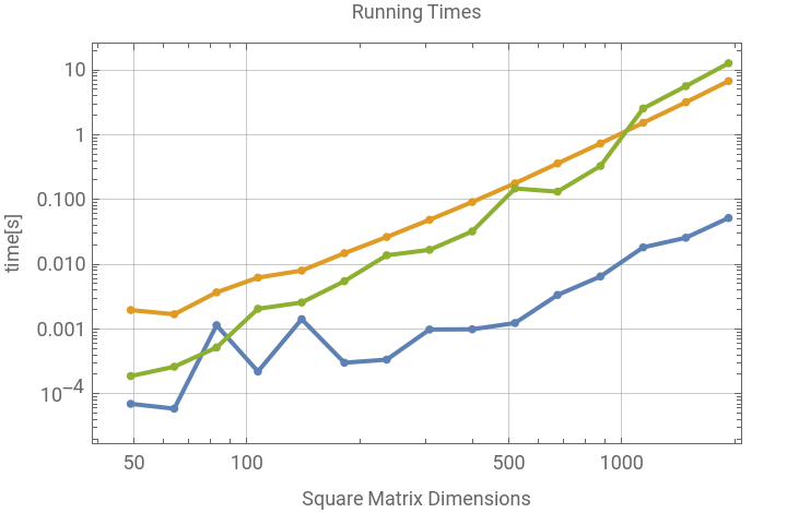


Note that the accumulated outer product becomes slower than the iterated inner product for n > 1000.
Summary
Summary
All three algorithms have a time complexity of O(n^3), which is apparent in the plot. That is, the time to multiply two n x n matrices takes K(n) n^3 seconds, where K(n) is bounded. The coefficient K(n) might change when thresholds of system parameters are crossed, such as vectorization limits in the math libraries or cache limits in the CPU. I suspect that’s what is happening when the outer-product method slows down for n > 1000 in the refactored versions. Outer[] has an internal, optimized nested for-loop. That’s why it beats nested For[] in Brian’s versions. And it beats the refactored Do[] for moderately large square matrices. However, the first two examples, in which the inner product was faster, suggest that determining the exact conditions under which outer is better than inner is going to be difficult.
To reiterate, the trials above were performed on a 2021 Macbook Pro M1 Max (32GB).