CITE THIS NOTEBOOK: Summation over the roots of the Zeta function in the critical strip by Oliver Seipel. Wolfram Community JAN 2 2023.
H. M. Edwards Riemann’s Zeta Function 1974, 2001, p.66/67: =γ+logπ+1-log2π≈0.0230357where the sum over ρ is in the order of increasing .This formula was known to Riemann, who used it in his computations of the root ρ.
∑
ρ
1
ρ
1
2
1
2
Imρ
I want to show how to compute this sum with Mathematica and some generalizations of the sum, i.e. , etc.
∑
ρ
1
ρ±1
∑
ρ
1
2
ρ
First approach
First approach
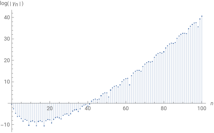
This defines the Stieltjes Gamma coefficients, which will appear later in the computations:
In[]:=
With[{expr=Zeta[z]},TraditionalForm[Row[{expr,"≈",Series[expr,{z,1,2}]}]]]
Out[]//TraditionalForm=
ζ(z)≈+-(z-1)++O()
1
z-1
γ
1
1
2
γ
2
2
(z-1)
3
(z-1)
Here are some first values:
In[]:=
N[StieltjesGamma[Range[0,3]]]
Out[]=
{0.577216,-0.0728158,-0.00969036,0.00205383}
Out[]=
The relationship between ζ(s) ans ζ(1-s) is known as the functional equation of the zeta function:
In[]:=
TraditionalForm[functionalequation=Zeta[s]==Zeta[1-s]Gamma[(1-s)/2]Gamma[s/2]]
s-1/2
π
Out[]//TraditionalForm=
ζ(s)ζ(1-s)Γ
s-
1
2
π
1-s
2
Γ
s
2
In[]:=
FullSimplify[functionalequation]
Out[]=
True
This is the definition of the RiemannXi function: which has the property:And has the same zeros as the non trivial zeros of and no poles, therefore:,
ξ(s)=(s-1)Γζ(s)
-s/2
π
s
2
s
2
ξ(s)=ξ(1-s)
ξ
ζ
ξ(s)=ξ(0)1-
∏
ρ
s
ρ
ξ(0)=1/2
logξ(s)=logξ(0)+log1-
∑
ρ
s
ρ
In[]:=
TraditionalForm[Row[{"ξ(s)=",RiemannXi[s]}]]
Out[]//TraditionalForm=
ξ(s)=(s-1)ζ(s)Γ+1
-s/2
π
s
2
This property of the Gamma function is useful:
In[]:=
FullSimplify[Gamma[s/2+1]==s/2Gamma[s/2]]
Out[]=
True
The logarithmic derivative of is logξ(s)=log1-===
ξ
s
∑
ρ
s
s
ρ
∑
ρ
1
s-ρ
∑
ρ
-1
ρ-s
-∑
ρ
1
ρ-s
Therefore we define the symbolic sum:
In[]:=
symbolicsum[s_,n_:1]:=Row"",
Σ
ρ
1
n
(ρ-s)
And the logarithmic derivative is:
In[]:=
TraditionalForm[expr=FullSimplify[D[Log[RiemannXi[s]],s]]==D[Log[ξ[s]],s]==-symbolicsum[s]]
Out[]//TraditionalForm=
′
ζ
ζ(s)
s(-log(π))+(s-1)+1+2+log(π)
(0)
ψ
s
2
2(s-1)
′
ξ
ξ(s)
Σ
ρ
1
ρ-s
There is no problem to replace by zero (otherwise we take the limit)
s
In[]:=
TraditionalForm[eqn=expr/.s->0]
Out[]//TraditionalForm=
1
2
′
ξ
ξ(0)
Σ
ρ
1
ρ
and therefore:=1++-log(2π)and also=1+-log2-logπ
∑
ρ
1
ρ
γ
2
logπ
2
∑
ρ
1
ρ
γ
2
1
2
Now we compute the second derivative:
In[]:=
TraditionalForm[expr=MultiplySides[FullSimplify[D[Log[RiemannXi[s]],{s,2}]]==D[Log[ξ[s]],{s,2}]==-symbolicsum[s,2],-1]]
Out[]//TraditionalForm=
-+-+1(s)-(s)
ζ(s)(s)-(s)
′′
ζ
2
′
ζ
2
ζ(s)
1
2
(s-1)
1
4
(1)
ψ
s
2
2
′
ξ
2
ξ(s)
′′
ξ
ξ(s)
Σ
ρ
1
2
(ρ-s)
In[]:=
TraditionalForm[Simplify[expr/.s->0]]
Out[]//TraditionalForm=
2+1+-(0)-ξ(0)(0)
γ
1
2
2
π
8
2
′
ξ
′′
ξ
2
ξ(0)
Σ
ρ
1
2
ρ
Now we compute the third derivative:
In[]:=
TraditionalForm[expr=MultiplySides[FullSimplify[D[Log[RiemannXi[s]],{s,3}]]==D[Log[ξ[s]],{s,3}]==-symbolicsum[s,3],-1]]
Out[]//TraditionalForm=
---+1-(s)-+
2(s)+(s)-3ζ(s)(s)(s)
3
′
ζ
(3)
ζ
2
ζ(s)
′
ζ
′′
ζ
3
ζ(s)
2
3
(s-1)
1
8
(2)
ψ
s
2
(3)
ξ
ξ(s)
2(s)
3
′
ξ
3
ξ(s)
3(s)(s)
′
ξ
′′
ξ
2
ξ(s)
Σ
ρ
1
3
(ρ-s)
In[]:=
TraditionalForm[FullSimplify[expr/.s->0]]
Out[]//TraditionalForm=
6+3-+2+2-(0)+2(0)-3ξ(0)(0)(0)
γ
1
γ
2
7ζ(3)
4
3
2
ξ(0)
(3)
ξ
3
′
ξ
′
ξ
′′
ξ
3
ξ(0)
Σ
ρ
1
3
ρ
This is turned into a function. (FullSimplify makes it slow, Limit is sometimes useful):
In[]:=
RiemannLimit[s0_,n_]:=symbolicsum[s0,n]==FullSimplifyLimitD[Log[RiemannXi[s]],{s,n}],s->s0
-1
(n-1)!
In[]:=
TraditionalForm[expr=RiemannLimit[0,1]]
Out[]//TraditionalForm=
Σ
ρ
1
ρ
1
2
In[]:=
N[expr]
Out[]=
Σ
ρ
1
ρ
In[]:=
TraditionalForm[RiemannLimit[-1,1]//FunctionExpand]
Out[]//TraditionalForm=
Σ
ρ
1
ρ+1
1
2
In[]:=
TraditionalForm[RiemannLimit[-1/2,1]//FunctionExpand]
Out[]//TraditionalForm=
Σ
ρ
1
ρ+
1
2
1
6
24π-
′
ζ
1
2
ζ
3
2
π
2
In[]:=
TraditionalForm[RiemannLimit[1,1]//FunctionExpand]
Second approach and numerical comparison.
Second approach and numerical comparison.
To check the sums numerically we compute the first 100 zeros pairwise:
Computation of the first derivative:
so we define:
And now we go recursively:
The numerical approximation is fine here:
The numerical approximation is fine here:
The numerical approximation is fine here:
Further Reading:
Further Reading:
https://arxiv.org/abs/1810.05198 (Carl Ludwid Siegel, 1932)
This is in English.
In 1859 Riemann (1826-1866) published his only paper on number theory. In this eight-page paper he obtained a formula for the number of primes less than or equal to a real number x, and revealed the deep connection between the distribution of primes and the zeros of an analytic function now called the Riemann Zeta Function. In the early 1930’s two related unpublished results from 1859 were found in Riemanns very rough notes by the great twentieth century mathematician and scholar, Carl Ludwig Siegel (1896-1981).
In his 1932 paper “Uber Riemanns Nachlass zur analytischen Zahlentheorie”(“On Riemann’s Nachlass for Analytic Number Theory”) Siegel presents these unpublished results and gives derivations he found in Riemann’s notes. The first is an asymptotic development, now called the Riemann-Siegel formula, for efficiently computing values of the Riemann Zeta Function. The second is a new integral representation of the zeta function. These results had not been rediscovered seventy years after Riemann. Thus, in 1932 the importance of Siegel’s paper was not only its contribution to the history of mathematics, but also its contribution to current research.
Riemann’s Zeta Function, H. M. Edwards, 1974. Republication 2001 Dover edition.
http://portail.mathdoc.fr/JMPA/PDF/JMPA_1893_ 4_ 9_A3 _ 0.pdf
This is in french.
J. HADAMARD
Etude sur les propriétés des fonctions entières et en particulier
d’une fonction considérée par Riemann
Journal de mathématiques pures et appliquées 4e
série, tome 9 (1893), p. 171-216.
This is in french.
J. HADAMARD
Etude sur les propriétés des fonctions entières et en particulier
d’une fonction considérée par Riemann
Journal de mathématiques pures et appliquées 4e
série, tome 9 (1893), p. 171-216.
https://de.wikisource.org/wiki/%C3 %9 Cber_die _Anzahl _der _Primzahlen _unter _einer _gegebenen _Gr % C3 % B6 % C3 %9 Fe
This is in German.
B. Riemann: Über die Anzahl der Primzahlen unter einer gegebenen Größe, Monatsberichte der Königlichen Preußischen Akademie der Wissenschaften zu Berlin. Aus dem Jahre 1859. S. 671–680.
This is in German.
B. Riemann: Über die Anzahl der Primzahlen unter einer gegebenen Größe, Monatsberichte der Königlichen Preußischen Akademie der Wissenschaften zu Berlin. Aus dem Jahre 1859. S. 671–680.