Introduction
Introduction
The theory of random walks provides one with a tool to understand and investigate the geometrical and dynamical properties of the underlying structure on which random walks takes place. For instance if the underlying structure is a graph, by investigating how far a random walk process has gone with respect to its initial position, one can extract useful information such as the connectivity between the nodes of the graph. WolframModels which have hypergraph representation, are interesting candidates to investigate the dynamics of such a process. This is of utmost importance, since the WolframModels have causal set representations. This causal sets thus can be faithfully embedded on Lorentzian manifolds. Thus in the continuum limit, the geometrical properties the manifold can be extracted from the embedded causal set and its algebraic structure and vice versa[4].Many properties of the random walk process are understood in terms of the site occupation and first-passage probabilities; with combinatorics and probability generating function of these quantities and knowing the probability transition matrix, such properties are studied for different variations of random walk processes. Here in this project the focus will be on the most generic type of random walk process called Pólya’s walk. Pólya’s walk is a random walk on a d-dimensional lattice which is homogeneous, which implies that the lattice is translationally invariant. Moreover, the Pólya’s walk is unbiased which implies the fact that, the probability of moving from one site to its neighbouring site is the same as if the walk was taking place the other way around. The formalism can be easily extended to the case where the underlying structure is graph. It is worth to mention that, in the case of graphs, the degree of nodes does not need necessarily to be the same as long as the translational invariance is not violated[1].The random walk theory not only provides one with insights about the geometry of the underlying structure and how a dynamical process would behave on such a structure, but naturally establishes a connection between those properties. One of such relations is the Alexander-Orbach (AO) relation which establishes a connection between the the Harmonic (spectral) dimension H, the dynamical exponent and the Hausdorff dimension D for a random walk process on a connected graph which is embedded in a Riemannian manifold. The relation asserts that [1, 2, 3]. (1)It is noteworthy to mention that the relation above does only hold true under conditions mentioned above. For instance, for the Koch curve, the AO relation remains valid on the contrary, it is violated for the random walk on Cantor dusts.The intention here is to address the validity of AO relation for hypergraphs and furthermore, if it is violated what are the possible extensions or considerations that have to be taken into account to propose a generalised relation such that it can establish connection between the geometry of the hypergraphs and the dynamics of the random walk process on them. This could potentially provide useful insights to establish isomorphism between the causal sets and the Lorentzian manifold on which they are embedded.
ν
w
H=2
Dν
w
Preliminaries
Preliminaries
A random walk of Pólya type on a hypergraph H=(V, E), where V is the set of all nodes and E is the set of hyperedges, is defined as random move from a given node to a node v at the step n+1 described via the following(v|)=p(v|)(|) (2)where (v|) is the occupation probability of being at node on the step given that the random walk has started from the initial node , and is the probability transition from the node to the node . The probability transition must by symmetric and moreover, it must be equally distributed amongst the neighbours of v, known as the degree of the node. Hence, if is a neighbour of v; we denote the degree of v with deg(v).The walk is said to be homogeneous (the graph is translationally invariant) if for every in V, (v|v) (which means the probability of being at node after step given that the random walk has started from the same node) is the same. This readily implies that no node is preferred to the other nodes.A hyperedge is a set of nodes that connects them. The number of nodes within each hyperedge is referred to as the degree of that hyperedge. This is a generalisation of the concept of edges in graphs that are incident on only two nodes, exactly. For instance a hyperedge of nodes has degree of three. To make it clearer for the reader, consider the following hypergraphsE(H) E(H) The hypergraph H is a normal graph. In other words, every hypergraph where the for every hyperedge within the set of hyperedges the degree is two, that hypergraph is a graph. Below are the plots of H on the left hand side and H on the right hand side.
′
v
P
n+1
v
0
Σ
′
v
′
v
P
n
′
v
v
0
P
n
v
0
v
th
n
v
0
p(v|)
′
v
′
v
v
p(v|)=
′
v
1
deg(v)
′
v
v
P
n
v
n
{1,2,3}
1
={{1,2,3},{2,3,4,5}}
2
={{1,2},{1,3},{2,3},{2,4},{2,5},{3,4},{3,5},{4,5}}
2
1
2
hypg1={{1,2,3},{2,3,4,5}};hypg2={{1,2},{1,3},{2,3},{2,4},{2,5},{3,4},{3,5},{4,5}};GraphicsRow[{ResourceFunction["HypergraphPlot"][hypg1,"SubsetBoundary"False],ResourceFunction["HypergraphPlot"][hypg2,"SubsetBoundary"False]}]
Out[]=
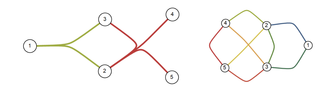
Their corresponding projected graphs are shown in the following figure. Note that the graph representation of these two hypergraphs are isomorphic.
graph1=UndirectedGraph[ResourceFunction["HypergraphToGraph"][hypg1]];graph2=UndirectedGraph[ResourceFunction["HypergraphToGraph"][hypg2]];GraphicsRow[{GraphPlot[graph1,VertexLabelsAutomatic,PlotLabelMaTeX["\\mathcal{G}_1"]],GraphPlot[graph2,VertexLabelsAutomatic,PlotLabelMaTeX["\\mathcal{G}_2"]]}]
Out[]=
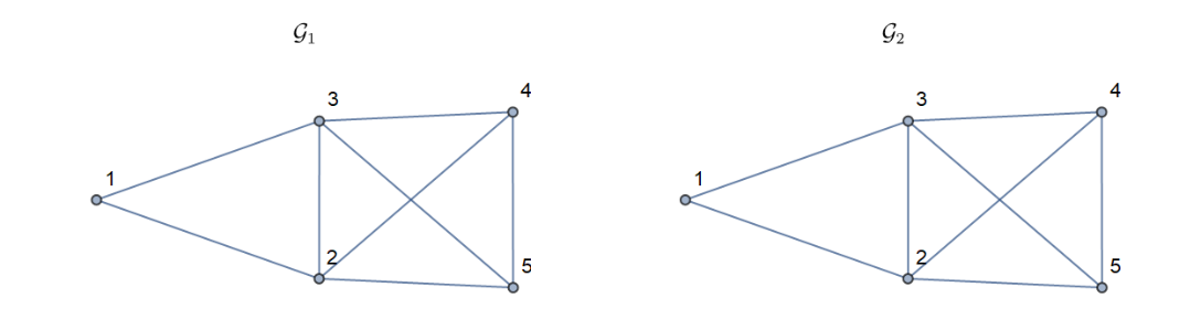
Thus, the random walk process on the projected graph of hypergraphs does not carry the same information, as during the transformation of the hypergraphs to their projected graphs, the information related to the hyperedges is lost. Therefore, a consideration has to be sought such that the structure of the hypergraphs are encoded in the probability transition matrix.
The natural distance on a graph is defined by the shortest path between two given nodes. It is denoted by d(u,v) for every pair of nodes u and v in V. If there is no path between the two nodes then d(u,v)=∞. Since in this project we are dealing with connected (hyper)graphs, the distance between every two given nodes is finite. Obviously d(v, v) = 0.
The natural distance on a graph is defined by the shortest path between two given nodes. It is denoted by d(u,v) for every pair of nodes u and v in V. If there is no path between the two nodes then d(u,v)=∞. Since in this project we are dealing with connected (hyper)graphs, the distance between every two given nodes is finite. Obviously d(v, v) = 0.
Probability Transition Matrix
Probability Transition Matrix
In order to take into account the structure of the hypergraphs, it is required to understand the connectivity between the nodes that belong to the same hyperedge set and those nodes that are connected via the overlap of other hyperedges. Assume the hypergraph H, notice that for the node 1, the probability of moving to the either node 2 or 3 is . That is also reflected on the projected graph G. Yet, the node 3 belongs to two different hyperedges; in the hyperedge , the probability to move to either node 1 or 2 is again while in the other hyperedge the probability to move to other three nodes 2, 3 and 5 is . Not surprisingly, it is seen that in G, node 3 is connected to all other nodes and the probability of moving to each one of them is . In order to incorporate the structure of the hypergraphs, initially it is required to define the incidence matrix[7]. Assuming the columns representing the hyperedges and the rows the nodes, the incidence matrix shows whether a node belongs to a specific hyperedge or not. It is said that a hyperedge is incident on a node if that node belongs to that given hyperedge. Therefore, the incidence matrix is an matrix where is the number of nodes in the set and is the number of hyperedges in . Thence, one can readily define the adjacency matrix and the hyperedge matrix by multiplying the transpose of the incidence matrix onto itself from right and left respectively[7]. For instance the incidence matrices for the hypergraphs H and H are given by the followings
1
1
2
1
{1,2,3}
1
2
{2,3,4,5}
1
3
1
1
4
nm
n
V
m
E
1
2
incM1=Transpose[{{1,1,1,0,0},{0,1,1,1,1}}]//MatrixFormincM2=Transpose[{{1,1,0,0,0},{1,0,1,0,0},{0,1,1,0,0},{0,1,0,1,0},{0,1,0,0,1},{0,0,1,1,0},{0,0,1,0,1},{0,0,0,1,1}}]//MatrixForm
Out[]//MatrixForm=
1 | 0 |
1 | 1 |
1 | 1 |
0 | 1 |
0 | 1 |
Random Walks on wm7714 WolfromWorld
Random Walks on wm7714 WolfromWorld
The wm7714 WolframModel is chosen to investigate the validity of the AO relation.
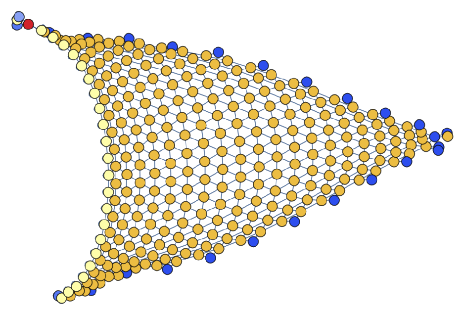
The figure depicted at top is the hypergraph representation of wm7714 whilst the one at the bottom demonstrates its undirected projected graph which preserves the geodesic distance between the nodes. After arriving at the probability transition matrix associated with the hypergraph representation of wm7714, it is straight forward to simulate random walk process on the undirected projected graph using discrete Markov process, needless to say that a random walk of Polya’s type is a Markov process. Here the initial condition is chosen such that the random walk process starts at node 1 and takes a path of length 1000. An ensemble of 500 of such walks is sampled.
Spectral Dimension and the Distinct Visited Nodes
Spectral Dimension and the Distinct Visited Nodes
which shows that the half of the spectral dimension has the value 0.86 and consequently the value 1.72 for H.
Dynamical Exponent
Dynamical Exponent
Hausdorff Dimension
Hausdorff Dimension
which yields a value of 2.004.
Validity of the AO relation
Validity of the AO relation
This bring us to the following conclusions
Conclusions and Future Directions
Conclusions and Future Directions
◼
What are the alternative generalised form of the AO relation that could establish a connection between the geometrical properties of the hypergraph and the dynamical behaviour of random walk on hypergraphs
◼
Is it required to generalise the notion of the Hausdorff dimension by taking into account the degree of each node. In other words, does the higher return occupation probability imply higher mass concentration?
◼
How to avoid the effect of the finiteness of the WolframModel. This can be addressed in two separate way (i) sample larger universes with WolframModel such that for a comparably shorter random walk processes the hypergraph seems to be infinite (ii) assert periodic boundary condition
◼
Another subtlety arises regarding the mode of the random walk. There are generally two modes of the random walk process; blind ant and myopic ant. The probability transition matrix deduced above corresponds to the myopic ant. At every step, the myopic ant takes a step to its neighbouring nodes whilst the blind ant has the possibility to stay on the node where it currently resides at. This is also commonly referred to as α-lazy random walk where 0< α <1 is the probability for the random walk to stay at the current node in its next step. It is known that the stationary distribution for these two walks reached differently see [8].
Acknowledgments
Acknowledgments
Mentor: Jon Lederman
I am grateful for the fruitful discussions and suggestions I had and received from my mentor Jon Lederman and the helps I received from Jonathan Gorard, Xerxes D. Arsiwala, Stephen Wolfram, Hatem Elshatlawy and Max Piskunov. Moreovery, I would like to thank all the organisers of the Wolfrom Physics Winter School WWS 2021 for their support and making it possible to carry out this project.
I am grateful for the fruitful discussions and suggestions I had and received from my mentor Jon Lederman and the helps I received from Jonathan Gorard, Xerxes D. Arsiwala, Stephen Wolfram, Hatem Elshatlawy and Max Piskunov. Moreovery, I would like to thank all the organisers of the Wolfrom Physics Winter School WWS 2021 for their support and making it possible to carry out this project.
References
References
◼
[1] Hughes, Barry D. Random walks and random environments: random walks. Vol. 1. Oxford University Press, 1995.
◼
[2] Hughes, Barry D. Random walks and random environments: random walks. Vol. 2. Oxford University Press, 1995.
◼
[3] Geoffrey Grimmett. Percolation. Springer Science & Business Media, 2013
◼
[4] Gorard, J., 2020. Algorithmic Causal Sets and the Wolfram Model. arXiv preprint arXiv:2011.12174.
◼
[5] Gorard, J., 2020. Some Relativistic and Gravitational Properties of the Wolfram Model. arXiv preprint arXiv:2004.14810.
◼
[6] Sokolov, I.M., 2016. What is the alternative to the Alexander–Orbach relation?. Journal of Physics A: Mathematical and Theoretical, 49(9), p.095003.
◼
[7] Carletti, T., Battiston, F., Cencetti, G. and Fanelli, D., 2020. Random walks on hypergraphs. Physical Review E, 101(2), p.022308.
◼
[8] Jacobs, D. and Nakanishi, H., 1990. Autocorrelation functions for discrete random walks on disordered lattice. Physical Review A, 41(2), p.706.