An optimization program designed to discover specific cellular automaton rules
In the domain of cellular automata (CA), the rule space exhibits exponential growth with respect to the number of states per cell. Consider the elementary cellular automaton with binary states: it encompasses 256 distinct rules, each capable of generating diverse spatiotemporal patterns. However, when extending to ternary states, the rule space experiences a dramatic expansion to approximately 7.63 trillion possible rules.
This astronomical increase in the rule space presents significant computational and analytical challenges. While the binary CA’s complete rule space has been extensively studied and classified, the ternary CA’s vast rule space renders exhaustive exploration computationally intractable. The identification of specific pattern-generating rules within this expansive space becomes particularly challenging, as the search space grows exponentially with the number of states.
This characteristic of cellular automata systems underscores the fundamental challenges in complex systems analysis and highlights the limitations of brute-force approaches in studying higher-order cellular automata configurations.
To address these challenges, we propose a novel algorithmic approach that leverages the intrinsic connectivity patterns between cellular automata rules. Our methodology establishes a traceable exploration framework that capitalizes on the inherent relationships among CA rules. The algorithm employs a fitness function to identify optimal rule configurations and pattern formations within the vast rule space.
Specifically, our approach introduces a network-based exploration paradigm where rules are interconnected based on their behavioral similarities and pattern-generating characteristics. By mapping these relationships, we create a navigable topology within the rule space, enabling more efficient and directed exploration compared to traditional exhaustive search methods.
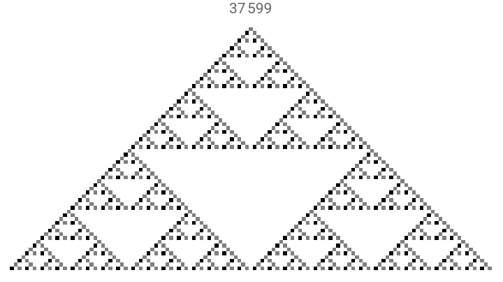
Here are various of three colors rules you can do to visualize it, just list some of them
In[]:=
Manipulate[Column[{RulePlot[CellularAutomaton[{rule,3,1}]],ArrayPlot[CellularAutomaton[{rule,3,1},{{1},0},step],PlotLabel->rule,Frame->None,Mesh->mesh]}],{{rule,30},0,3^10,1},{step,5,100,1},{{mesh,None},{True,None}}]
Out[]=


Fitness function:
In our investigation of cellular automata patterns, we focus specifically on identifying and quantifying “persistent local patterns” (PLPs). These patterns are characterized by localized oscillatory behaviors within a globally stable lattice - where dynamic evolution occurs only in confined regions while the surrounding cells remain static.
To systematically identify these patterns, we develop a fitness function that quantifies the essential characteristics of PLPs:
Spatial localization of dynamic activity: periodicity, Stability of surrounding regions and Pattern persistence
This fitness function transforms qualitative pattern recognition into a quantifiable optimization problem, providing a mathematical framework for automated pattern detection and evaluation within cellular automata systems.
middlePart[l:{___Integer}]:=Module[{leadingZeros=Length[TakeWhile[l,#==0&]]},{leadingZeros,Replace[l,{{___,x:Except[0],Longest[y___],z:Except[0],___}:>{x,y,z},{___,x:Except[0],___}:>{x},_->{}}]}](*Usage:*middlePart[{0,0,1,0,2,0,3,0}output:{2,{1,0,2,0,3}}*)deleteRange[l_List,{start_Integer,end_Integer}]:=Delete[l,List/@Range[start,end]]sequenceReplaceAt[l_List,replacement_List,start_Integer]:=Insert[deleteRange[l,{start,start+Length[replacement]-1}],Splice[replacement],start]sequenceDistance[smaller:{___Integer},larger:{___Integer}]:=Min@Table[HammingDistance[larger,sequenceReplaceAt[ConstantArray[0,Length[larger]],smaller,i]],{i,1,Length[larger]-Length[smaller]+1}]stepDistance[target:{___Integer}][step:{___Integer}]:=stepDistance[step,target]stepDistance[step_,target_]:=sequenceDistance[middlePart[step][[2]],target]fitness[cAHist:{{___Integer}...},target:{___Integer}]:={-Min[stepDistance[target]/@cAHist],First[First[MinPosition[stepDistance[target]/@cAHist]]]}NumofZero[hist_,index_]:={middlePart[hist[[index]]][[1]]}ReturnLocation[hist_,target_]:={result=fitness[hist,target];x=NumofZero[hist,result[[2]]][[1]];y=result[[2]];x,y+1}
Overall, the core purpose of this function system is to locate the spatiotemporal coordinates of specific patterns within the evolutionary history of cellular automata - specifically identifying at which time step (y-coordinate) a target pattern appears and its horizontal position offset (x-coordinate, represented by the number of leading zeros) within that time step, where all other functions such as pattern extraction (middlePart), sequence distance calculation (sequenceDistance), and fitness evaluation (fitness) serve as auxiliary tools to achieve this ultimate goal.
The middlePart function implements a pattern extraction mechanism that processes integer sequences to identify their essential non-zero components. This function returns a tuple containing two elements: the count of leading zeros and the extracted non-zero subsequence. The extraction process eliminates peripheral zeros while preserving the internal structure of the sequence. For instance, given an input sequence {0,0,1,0,2,0,3,0}, the function returns {2,{1,0,2,0,3}}, where 2 represents the number of leading zeros, and the second element captures the core pattern.
The deleteRange function implements an interval deletion operation on sequences. It accepts a source sequence and a deletion interval specified by start and end positions. The function systematically removes elements within the specified interval by converting the range into a list of deletion positions, effectively producing a new sequence with the designated section removed.
The sequenceReplaceAt function performs a sophisticated sequence substitution operation. It executes a two-phase process: first removing elements from the specified position range in the original sequence, then inserting the replacement subsequence at the designated start position. This operation maintains sequence integrity while implementing the desired substitution.
The sequenceDistance function computes the minimal Hamming distance between two sequences of different lengths. It employs a sliding window approach, embedding the shorter sequence within a zero-padded sequence of equal length to the longer sequence. The function systematically evaluates all possible alignments, returning the minimum Hamming distance achieved across all positions.
The stepDistance function serves as a metric for comparing cellular automata evolution steps with target patterns. It first processes the evolution step through the middlePart function to extract the relevant pattern, then computes the sequence distance between this extracted pattern and the target sequence. This function effectively quantifies the similarity between evolutionary states and desired patterns.
The fitness function implements a comprehensive evaluation mechanism for analyzing the evolutionary history of a cellular automaton against a target pattern. It computes a dual-metric assessment by first determining the minimum step distance across all historical states, then negating this value to create a fitness score where higher values indicate better pattern matches. Simultaneously, it identifies the temporal index at which this optimal match occurs. The function returns these metrics as a tuple, providing both qualitative (fitness) and temporal (position) information about pattern emergence.
The NumofZero function performs a specialized analysis of spatial positioning within cellular automaton states. By extracting the count of leading zeros from a specific historical state, it provides crucial information about the spatial offset of patterns within the cellular lattice. This measurement becomes particularly significant when tracking pattern migration and positioning throughout the automaton’s evolution.
The ReturnLocation function synthesizes spatial and temporal pattern analysis into a unified coordinate system. It begins by computing fitness metrics for the evolutionary history, then extracts the spatial positioning information from the optimal matching state. The function culminates in returning a coordinate pair that encodes both spatial and temporal information about pattern occurrence. The spatial coordinate (x) represents the pattern’s position within the lattice through its leading zero count, while the temporal coordinate (y+1) indicates the adjusted time step at which the pattern manifests.
This integrated suite of functions establishes a sophisticated mathematical framework for pattern analysis in cellular automata systems. The framework enables precise pattern extraction, normalization, and comparison through distance metrics, while simultaneously tracking the spatiotemporal evolution of these patterns. Through this comprehensive approach, the system facilitates detailed analysis of pattern formation, migration, and self-organization phenomena within cellular automata. The mathematical rigor of the implementation supports both theoretical investigations and practical applications in studying emergent behaviors in discrete dynamical systems.
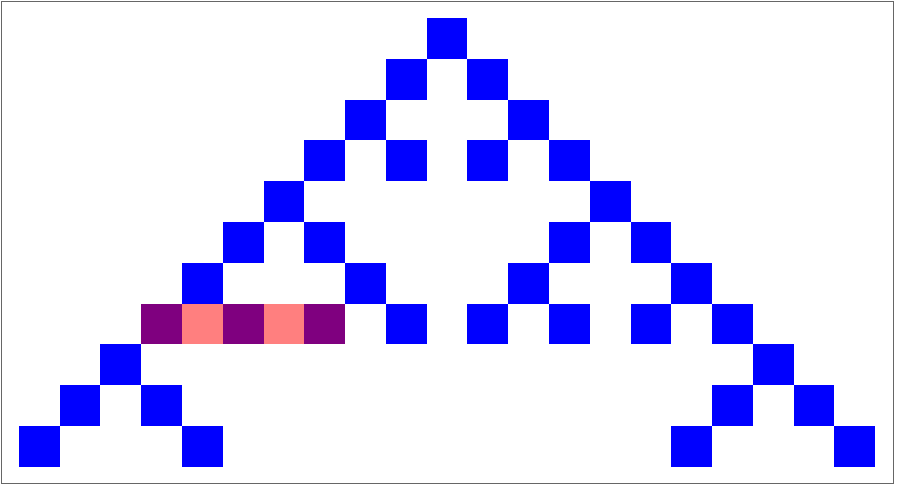
To visualize the fitness trajectories more effectively, we implement the GraphPlotCellular function, which provides precise spatial mapping of the pattern sequences within the cellular automaton’s evolution. The demonstration reveals several distinct pattern series, offering direct visual confirmation of our numerical pattern detection results.
GraphPlotCellular[hist_,cord_,Target_]:=Module{highlightRow,startCol,endCol,highlightCoords,dims},highlightRow=cord[[1]];startCol=cord[[2]];endCol=Min[Length[Target]+1,Length[hist[[1]]]]; If[highlightRow>Length[hist],Return[ArrayPlot[hist/.{0->White,1->Blue}]]]; highlightCoords=Table[{highlightRow,c},{c,startCol,endCol}]; highlightCoords=Select[highlightCoords,1<=#[[1]]<=Length[hist]&&1<=#[[2]]<=Length[hist[[1]]]&];ArrayPlot[MapAt[Blend[{#,Red},.5]&,hist/.{0->White,1->Blue},highlightCoords]]hist=CellularAutomaton[{24789,3,1},{{1},0},10];Target={1,0,1,0,1,0,1};Print["Here is the result"]result=fitness[hist,Target]Print["Here is the location"]ReturnLocation[hist,Target]GraphPlotCellular[hist,ReturnLocation[hist,Target],Target]
Network Neighbor Searching Algorithm (NNSA)
The algorithm leverages the topological structure of Boolean hypercube to conduct systematic rule exploration in search of optimal configurations that align with target specifications. The methodology employs a dual-strategy approach: deterministic traversal through hypercube vertices complemented by stochastic initialization to mitigate local optima convergence.The Boolean hypercube framework provides a natural representation for the rule space, where each vertex corresponds to a unique rule configuration, and edges represent single-bit transitions between rules. This geometric interpretation facilitates efficient navigation through the solution space while maintaining the inherent binary relationships between adjacent configurations.To address the challenge of local optimality traps, the algorithm implements a hybrid search strategy. The primary component involves systematic exploration of the hypercube structure, exploiting the inherent connectivity patterns to identify promising rule candidates. This is augmented by a randomized initialization mechanism that introduces exploration of previously unexplored regions of the search space, thereby enhancing the algorithm’s capability to escape local maxima and discover globally optimal solutions.
UndirectedGraph[Catenate[Table[#->MapAt[1-#&,#,i],{i,Length[#]}]&/@Tuples[{1,0},7]],EdgeStyle->Opacity[.4,Gray],VertexSize->0,VertexLabels->{x_:>Placed[ArrayPlot[{Append[x,0]},Mesh->True,ImageSize->40],Center]}]
In[]:=
RandomInitialState[]:=RandomInteger[{1,3^10},10](*generatethemutations*)myRandomChoice[{}]={};myRandomChoice[l_List]:=RandomChoice[l,1];GenerateMutations[rule_,k_]:=FromDigits[#,k]&/@DeleteDuplicates[Flatten[Table[NestList[MapAt[Mod[#+1,k]&,#,i]&,IntegerDigits[rule,k,Length[IntegerDigits[k^k^k-1,k]]],k],{i,1,Length[IntegerDigits[k^k^k-1,k]]}],1]]NewList[num_]:=DeleteCases[GenerateMutations[num,3],num]GetPerfectRule[rules_,Series_]:=Module[{fitness,bestIndices,dict,PerfectRulelist},Print["Starting to calculate fitness for ",Length[rules]," rules..."];fitness=Table[If[Mod[i,10]==0,Print["Progress: ",Round[100.0*i/Length[rules],0.1],"%"]];fitnessWithRule[rules[[i]],Series],{i,Length[rules]}];Print["Fitness calculation completed, maximum fitness: ",Max[fitness]];If[Max[fitness]<0,(*Ifallvaluesarelessthan0,returnthethreeclosestto0*)bestIndices=Ordering[fitness,-3];dict=Association[MapThread[Rule,{rules,fitness}]];PerfectRulelist=rules[[Join[bestIndices,myRandomChoice@Complement[Range[Length[rules]],bestIndices]]]];Print["Didn't find anything"];Print[PerfectRulelist];Print["Best rules and their fitness values:"];Print[Association[Rule[#,dict[#]]&/@PerfectRulelist]];{False,PerfectRulelist},(*else*)dict=Association[MapThread[Rule,{rules,fitness}]];PerfectRulelist=Select[Keys[dict],dict[#]>=0&];Print["Find some good example"];Print["Rules and their fitness values:"];Print[Association[Rule[#,dict[#]]&/@PerfectRulelist]];{True,PerfectRulelist}]]IterateUntilPerfect[initialRules_,Series_,maxIterations_:10]:=Module[{currentResult,iteration=1,rules=initialRules,testedRules={}},(*AddtestedRulestostoretestedrules*)currentResult=GetPerfectRule[rules,Series];testedRules=Union[testedRules,rules];(*Addtotestedrulesset*)While[currentResult[[1]]==False&&iteration<maxIterations,rules=Flatten[NewList/@currentResult[[2]]];(*Removepreviouslytestedrules*)rules=DeleteDuplicates[Select[rules,!MemberQ[testedRules,#]&]];Print["Number of tested rules: ",Length[testedRules]];Print["Number of new rules: ",Length[rules]];If[Length[rules]==0,Print["No new rules to test!"];Break[];];Print["Evaluating new rules..."];currentResult=GetPerfectRule[rules,Series];testedRules=Union[testedRules,rules];(*Updatetestedrulesset*)Print["Evaluation completed"];iteration++;];currentResult[[2]]]FindYourSeries[Series_]:=Module[{rules,FinalList},rules=RandomInitialState[];FinalList=IterateUntilPerfect[rules,Series];FinalList]
This set of functions implements a rule search system based on evolutionary algorithms. The core concept involves searching for rules that meet specific conditions within a rule space by simulating the mutation and natural selection processes found in biological evolution.
Initially, the RandomInitialState function initializes the rule set by generating 10 random integers within the range [1, 3^10]. These random numbers serve as the initial population, representing starting points in the search space. The myRandomChoice function acts as an auxiliary tool, implementing a mechanism for single element random selection.
Regarding mutation generation, the GenerateMutations function implements the rule variation mechanism. It takes a rule and a base number k as input, generating all possible single-point mutations by systematically altering each digit of the rule. This process simulates gene mutation in biological evolution. The NewList function further refines these mutations by excluding the original rule to ensure population diversity.
The GetPerfectRule function assumes the role of fitness evaluation. It calculates the fitness value for each rule and selects suitable rules based on preset criteria. When no rules fully meeting the requirements are found, it selects the rules closest to the target as the foundation for the next generation. This process mirrors the survival of the fittest principle in natural selection.
The IterateUntilPerfect function implements the iterative control of the entire evolutionary process. It maintains a set of tested rules, gradually converging toward target rules through continuous generation of new mutations and evaluation of their fitness. This function also includes mechanisms to prevent duplicate testing, improving search efficiency.
Finally, the FindYourSeries function serves as the entry point for the entire system, encapsulating the complete process from initialization to final result acquisition. It initiates random initialization and then seeks rule sets meeting the requirements through an iterative evolutionary process.
Reference:
1. Wolfram, S. (2024, May 3). Why does biological evolution work? A minimal model for biological evolution and other adaptive processes. Stephen Wolfram Writings. https://writings.stephenwolfram.com/2024/05/why-does-biological-evolution-work-a-minimal-model-for-biological-evolution-and-other-adaptive-processes/
2.
2.