The NCBI Tree of Life – a 57-species sample, built from Wolfram's curated taxonomy and drawn as a circular cladogram (root ⊳ phylum ⊳ class ⊳ order ⊳ family ⊳ species), branches coloured by class. This single tree is the only structure the method needs. Encode each leaf by its root-to-leaf child indices as the digits of a base-p integer, and the p-adic distance between two leaves becomes p raised to minus the depth of their lowest common ancestor – the tree's own nesting, captured exactly as its canonical ultrametric. Everything downstream – a tuning-free nearest-neighbour classifier, coarse-level predictions provably stable under label noise, and a Dendrogram that rebuilds the taxonomy exactly – is read off this picture for free. The same recipe reproduces ICD-10 diagnostic codes, Library of Congress call numbers, IP routing tables, and map tiles.
Pour a stream of data labels into almost any real classification problem and they arrange themselves on a tree: a disease code sits in a category, inside a block, inside a chapter; a species sits in a genus, in a family, in an order. The natural way to ask “how similar are two leaves?” is to walk back up the tree until their paths meet. Remarkably, that intuitive tree distance is not a heuristic at all – it is a 130-year-old object from number theory, the p-adic absolute value of Kurt Hensel (1897), wearing a disguise.
The idea in one line. Encode each leaf as an integer whose base- digits are its child-indices from the root; then the p-adic distance between the encoded integers equals – the depth of their lowest common ancestor, on the nose. (This is the tree's canonical ultrametric, the one whose balls are its subtrees – not the additive root-to-root path length.)
p
d(x,y)=
p
-(x-y)
v
p
p
-depth(LCA)
p
Why it matters. Most machine-learning machinery treats labels as structureless one-hot vectors, so predicting “lion” for a tiger is scored exactly as wrong as predicting “octopus”. The p-adic metric puts the hierarchy back. A plain 1-nearest-neighbour classifier under it inherits the taxonomy for free: no training, no hyper-parameters, no learned embedding – and, because the distance is an ultrametric, its coarse-level predictions are provably stable under leaf-level label noise (§7). On 162 real leaves from three live taxonomies it matches or beats the Euclidean and Hamming baselines at every level – with the widest margins at the intermediate levels – and (§9) it makes Wolfram Language's own Dendrogram reconstruct the taxonomy exactly while automatic Classify scores barely above chance on the same encodings.
What this post does from scratch in the Wolfram Language. Define the p-adic primitives in five lines; prove the ultrametric facts that make everything work; encode three real hierarchies (WHO ICD-10, the NCBI Tree of Life, and Library of Congress call numbers); run a 200-split nearest-neighbour benchmark and a label-noise sweep; compare head-to-head with the built-in Nearest, Dendrogram and Classify; and finally apply the very same construction to IP routing tables, GeoHash map tiles, and file-system paths.
All the heavy lifting lives in one companion file, padic_taxonomy.wl – the only file you need beside this notebook. It ships the p-adic primitives, the three baked-in taxonomy datasets, the precomputed 200-split results, and every figure generator, so the post opens instantly with no downloads and no API keys. Each displayed result is a one-liner sitting directly above its (pre-computed) output. Evaluate the cell below once, then any other cell will Just Work:
Get@FileNameJoin[{NotebookDirectory[],"padic_taxonomy.wl"}]
To redraw the hero tree, evaluate ncbiRadialFigure[]; for an animated dive into the matching tree of p-adic balls, evaluate ListAnimate @ padicZoomFrames[3].
1. Why this is interesting
1. Why this is interesting
Almost every classification problem in the wild lives on a tree. Diagnostic codes (ICD-10), tree-of-life taxa (NCBI), library call numbers (LCC), industry codes (NACE / SIC), accounting charts, organisational hierarchies, directory structures, ontologies (GO, MeSH, SNOMED) – all of them have a root, parents, children, leaves, and the natural way to say "these two leaves are similar" is to walk back up the tree and ask: how deep is their deepest common ancestor?
Yet most off-the-shelf machine-learning machinery treats labels as one-hot vectors with no structure: predicting "lion" when the truth is "tiger" is exactly as wrong as predicting "common octopus". That's strange. Hierarchical-softmax architectures, tree-structured loss functions, Wu-Palmer / Resnik path similarities in NLP, and various forms of label smoothing exist precisely to fix this – but they're all bespoke, all require tuning, and all sit on top of a learned embedding.
The observation in this note is that the canonical ultrametric on any rooted taxonomy – the one that ranks leaf pairs by the depth of their lowest common ancestor – is literally the p-adic distance after a one-line encoding, and that as a consequence a plain 1-NN classifier inherits the taxonomy structure for free: hyperparameter-free, training-free, embedding-free, and – as a corollary of the ultrametric property – noise-immune at coarse levels.
We make this completely concrete on three real classifications drawn from Wolfram's curated knowledgebase and from public taxonomy specifications. All code below is plain wolframscript-able Wolfram Language; the longest primitive is six lines.
2. The p-adic absolute value
2. The p-adic absolute value
2.1 Valuation, norm, distance
2.1 Valuation, norm, distance
Pick once and for all a prime . For a non-zero integer , write
p
n
n=·m,gcd(m,p)=1,k≥0
k
p
The integer (the multiplicity with which divides ) is the p-adic valuation (n). The p-adic absolute value of is then defined as
k
p
n
v
p
n
|n|
p
-(n)
v
p
p
with the conventions (0) = and = . Small numbers (in the p-adic sense) are the ones that are highly divisible by : , , , … shrink towards zero. Numbers prime to all have norm exactly 1.
v
p
∞
|0|
p
0
p
p
2
p
3
p
p
The point of the definition is that is not merely a gadget but a genuine absolute value on : it is non-negative, vanishes only at 0, and – crucially – respects multiplication. This last fact is what ties it to the arithmetic of and is where the primality of first earns its keep.
|·|
p
p
Lemma 1. (Multiplicativity.) For all non-zero , ∈ , (ab)=(a)+(b), hence = ·. Consequently is a multiplicative absolute value on .
a
b
v
p
v
p
v
p
|ab|
p
|a|
p
|b|
p
|·|
p
Proof. By unique factorisation in write and with . Then . Because is prime, divides neither nor , and a prime that divides a product divides one of the factors; therefore does not divide , so (ab) = . Raising to the negation of both sides gives = ·. The extension to by = / is then forced and well defined. ■
a=m
i
p
b=n
j
p
gcd(m,p)=gcd(n,p)=1
ab=(mn)
i+j
p
p
p
m
n
p
mn
v
p
i+j
p
|ab|
p
|a|
p
|b|
p
|a/b|
p
|a|
p
|b|
p
Remark. Primality is genuinely used. For a composite base such as , IntegerExponent still makes sense but is no longer additive: (2)=0 while (2·2)=(4)=1≠0, so is not multiplicative and is not a domain. As we will see in §3, the prefix-distance we build is nonetheless a perfectly good ultrametric for any integer radix ≥ 2 – the ultrametric inequality needs only (x+y)≥min, which holds for every base. Primality buys two extra things we want: multiplicativity (Lemma 1) and, through it, the complete field and the Ostrowski uniqueness of §2.2. In the taxonomy application we therefore always pick prime with ≥ (maximum branching factor).
4
v
4
v
4
v
4
|·|
4
4
v
b
p
p
p-1
The induced distance (x, y) = is a genuine metric on (and extends to a metric on by = /). It satisfies an inequality strictly stronger than the ordinary triangle inequality:
d
p
|x-y|
p
|a/b|
p
|a|
p
|b|
p
d(x,z)≤max(d(x,y),d(y,z))
p
p
p
This is the strong (or ultrametric) triangle inequality, and it changes geometry profoundly: every triangle has two long sides and they are equal; every point of a ball is its centre; balls are clopen (simultaneously closed and open); the closed balls form a tree under inclusion. The last property is the one we will harvest.
strongTriangleFigure[]
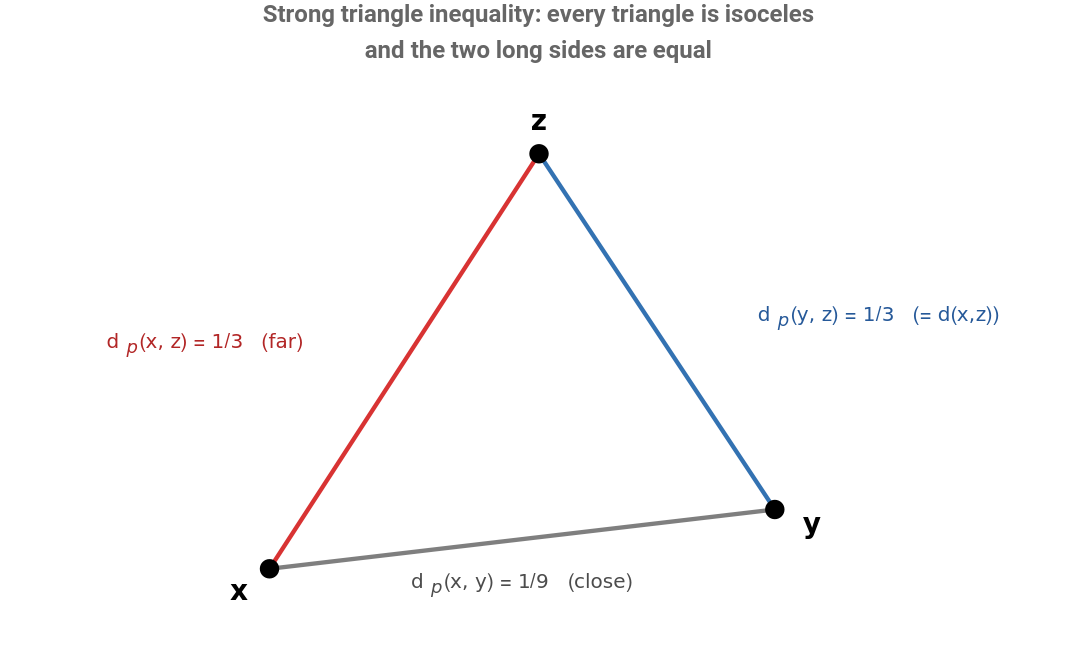
Figure 1. The strong triangle inequality in pictures. In a p-adic triangle, if y sits much closer to x than z does, then y is automatically the same p-adic distance from z as x is. The two longer sides of every triangle are equal.
2.2 Ostrowski: the p-adic absolute values are the only siblings of the Euclidean one
2.2 Ostrowski: the p-adic absolute values are the only siblings of the Euclidean one
The p-adic absolute values are not arbitrary toys. Ostrowski's theorem (1916) states that every non-trivial absolute value on is equivalent either to the usual Euclidean absolute value or to for exactly one prime . Concretely:
|·|
|·|
p
p
{ absolute values on } / ∼ = { trivial, | · | = Euclidean, | · |p for prime p }
So as soon as we want a non-trivial way to measure 'size' on the rationals that respects multiplication, we are forced to choose between the familiar Archimedean (Euclidean) world and exactly one p-adic world per prime. The p-adic absolute values are not curiosities; they are the only other places of – the natural non-Archimedean siblings of the ruler we already know.Each yields, by Cauchy completion, a topologically complete field which contains densely. The subring of p-adic integers consists of those -numbers whose Hensel expansion +p++... has only non-negative powers of . Geometrically, is a Cantor-like fractal:
|·|
p
p
p
p
a
0
a
1
a
2
2
p
p
p
padicBallsFigure[]
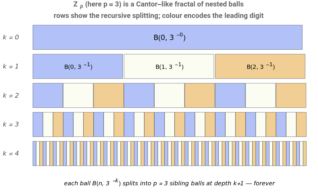
Figure 2. The p-adic integers Z_p, here for p = 3, are a Cantor-like nested tree of balls. The top row is the ball B(0, 1) = Z_p itself; the next row is its decomposition into three sibling balls B(0, 1/p), B(1, 1/p), B(2, 1/p); each of those in turn splits into p smaller balls, and so on forever. The colour encodes the leading digit a_0 of the Hensel expansion.
2.3 Completeness, Hensel expansions, and Hensel's lemma
2.3 Completeness, Hensel expansions, and Hensel's lemma
Definition 1. The field of p-adic numbers is the completion of with respect to : its elements are equivalence classes of -Cauchy sequences of rationals, two sequences being identified when their difference tends -to-zero. The p-adic integers are its closed unit ball ={x∈:|x|≤1}.
p
d
p
d
p
d
p
p
p
p
Every has a unique Hensel expansion
x∈,x≠0
p
x=,∈{0,…,p-1},≠0
∞
∑
i=-m
a
i
i
p
a
i
a
-m
and exactly when (only non-negative powers of ). The contrast with the real numbers is the whole story in one line: a decimal expansion runs infinitely to the right (adding ever-smaller corrections ), whereas a Hensel expansion runs infinitely to the left (adding ever-smaller -adic corrections , because is small). A four-line routine reads the digits off any rational:
x∈
p
m≤0
p
Archimedean
-i
10
p
i
p
||=
i
p
p
-i
p
HenselDigits[r_Rational|r_Integer,p_,n_]:=Module[{x=r,d,out={}},Do[d=Mod[Numerator[x]*PowerMod[Denominator[x],-1,p],p];AppendTo[out,d];x=(x-d)/p,{n}];out(*low-orderdigitfirst*)];HenselDigits[1/3,7,8]
{5,4,4,4,4,4,4,4}
So in . Just as in a number is rational iff its decimal expansion is eventually periodic, a -adic number lies in iff its Hensel expansion is eventually periodic – here the repeating block is simply .
1/3=5+4·7+4·+…
2
7
7
p
4
The single deepest fact about is that approximate solutions of polynomial equations can be refined one digit at a time – a -adic Newton's method:
p
p
Theorem 1. (Hensel's lemma, 1897.) Let and suppose some ∈ satisfies while ()≢0 . Then there is a unique with and .
f∈[x]
p
a
0
p
f()≡0
a
0
(modp)
′
f
a
0
(modp)
a∈
p
f(a)=0
a≡
a
0
(modp)
In words: a simple root modulo bootstraps to a genuine root in . For example +1 has the root mod 5 (=4≡-1), and , so is a square in . We lift it digit by digit with Newton's iteration modulo growing powers of 5:
p
p
2
x
x=2
2
2
2x≢0
-1
5
x→x-f(x)/(x)
′
f
HenselLift[p_,k_]:=Module[{x=2},(*rootofx^2+1mod5,thenlift*)Do[x=Mod[x-(x^2+1)*PowerMod[2x,-1,p^j],p^j],{j,2,k}];x];With[{r=HenselLift[5,8]},{r,Mod[r^2,5^8],Mod[-1,5^8]}]
Remark. A note on the software: contrary to a common belief, Wolfram Language 15 does not ship a built-in PadicNumber constructor; the expansions above are computed from first principles with PowerMod and IntegerExponent, both of which are core. Everything in this notebook is therefore self-contained number theory, not a library call.
2.4 The primitives in five lines of Wolfram Language
2.4 The primitives in five lines of Wolfram Language
PadicValuation[0, _] := Infinity;
PadicValuation[n_Integer, p_Integer] := IntegerExponent[n, p];
PadicAbs[0, _] := 0;
PadicAbs[n_Integer, p_Integer] := p^(-IntegerExponent[n, p]);
PadicDistance[x_Integer, y_Integer, p_Integer] := PadicAbs[x - y, p];
PadicValuation[0, _] := Infinity;
PadicValuation[n_Integer, p_Integer] := IntegerExponent[n, p];
PadicAbs[0, _] := 0;
PadicAbs[n_Integer, p_Integer] := p^(-IntegerExponent[n, p]);
PadicDistance[x_Integer, y_Integer, p_Integer] := PadicAbs[x - y, p];
A first sanity check:
3. The ultrametric property, explicitly
3. The ultrametric property, explicitly
3.1 The ultrametric inequality
3.1 The ultrametric inequality
3.2 Balls are clopen, and the balls form a tree
3.2 Balls are clopen, and the balls form a tree
Lemma 4 is the structural heart of the paper: the metric already carries a tree. The taxonomy we feed in will turn out to be precisely this tree of balls (§4), so everything an ultrametric knows about balls becomes a statement about the taxonomy for free.
4. A tree is a p-adic number system in disguise
4. A tree is a p-adic number system in disguise
4.1 The path-encoding
4.1 The path-encoding
4.2 The fundamental identification
4.2 The fundamental identification
Figure 3. Worked example at p = 3, depth = 3. The leaves x, y, z, w receive integer encodings 13, 22, 16, 14 respectively. d_3(x, y) = 1/9 because x and y share the two top levels of their path; d_3(x, z) = 1/3 because they share only the root edge; d_3(x, w) = 1 because they share nothing. The red trail marks the shared prefix of x and y; the p-adic distance is just p^{-(length of red trail)}.
4.3 Implementation in Wolfram Language
4.3 Implementation in Wolfram Language
The full encoder is two real lines of code:
EncodePath[path_List, p_Integer, depth_Integer] := Module[{padded},
padded = Join[path, ConstantArray[0, depth - Length[path]]];
Sum[padded[[i]] * p^(i - 1), {i, 1, depth}]
];
EncodePath[path_List, p_Integer, depth_Integer] := Module[{padded},
padded = Join[path, ConstantArray[0, depth - Length[path]]];
Sum[padded[[i]] * p^(i - 1), {i, 1, depth}]
];
Re-deriving the worked example from Figure 3:
5. Three real taxonomies
5. Three real taxonomies
We apply the construction to three openly-available hierarchical classifications, of widely differing depth and branching:
5.1 ICD-10 (WHO, International Classification of Diseases)
5.1 ICD-10 (WHO, International Classification of Diseases)
Figure 4. Chapter I of ICD-10 (certain infectious & parasitic diseases) viewed as a 4-level rooted tree. Each red leaf is a 4-character ICD-10 code, each grey interior node is a chapter / block / 3-character category. After our encoding, the p-adic distance between any two red leaves is p^{-(root-depth of their deepest common ancestor)}.
5.2 NCBI Tree of Life
5.2 NCBI Tree of Life
Figure 5. The mammals slice of our NCBI sample (class → order → family → species), 35 species across 6 orders. The tree structure is what determines the p-adic distance: e.g. lion and tiger are at p-adic distance p^{-6} (they share kingdom, phylum, class, order, family, genus); lion and gray wolf are at p^{-4} (share through order Carnivora); lion and human are at p^{-3} (share through class Mammalia).
We can verify those numbers by direct computation. The encoded integers for lion, tiger, gray wolf, human and honey bee from our pipeline are:
Reading off this matrix: lion and tiger are the most similar (same genus Panthera); lion and wolf are next (same order Carnivora); lion and human further (same class Mammalia); honey bee is maximally far from any mammal (different phylum already at the level of arthropods vs chordates). The numbers encode the taxonomy exactly.
5.3 Library of Congress Classification (LCC)
5.3 Library of Congress Classification (LCC)
5.4 Why the encoding really is the natural thing
5.4 Why the encoding really is the natural thing
The distance matrix induced by the encoding is striking when visualised:
Figure 6. Distance matrices on 28 ICD-10 leaves drawn from chapters I (infectious diseases) and II (neoplasms). Left: p-adic distance – the ultrametric block structure exactly mirrors the taxonomy (chapter blocks at the outer level, sub-blocks within each chapter, sibling pairs at the innermost level). Right: ordinary Euclidean distance on the base-p digit vector – noisy and largely uninformative. The p-adic matrix is literally the taxonomy's adjacency-style cluster structure, computed from the integer encoding alone.
6. 1-nearest-neighbour classification, three flavours
6. 1-nearest-neighbour classification, three flavours
◼
Euclidean on the same digit vector — the most generic baseline.
Implementing all three in WL is trivial. The p-adic version uses Wolfram's built-in Nearest with our custom distance function:
Figure 7. Hierarchical 1-NN accuracy as a function of ancestor depth k (counted from the root) for the three taxonomies, 200-split means with empirical 95% intervals (2.5–97.5 across-split percentiles). p-adic distance (red) dominates Hamming (blue) and Euclidean (green) at every single coarse level of every taxonomy. The rightmost depth in each panel is the exact leaf, where no method can recover a held-out point and every method scores 0.
Headline numbers:
◼
ICD-10 chapter prediction (k = 1): p-adic 99.4% vs Hamming 51.% vs Euclidean 65.4%.
◼
NCBI class prediction (k = 3): p-adic 90.9% vs Hamming 79.4% vs Euclidean 73.8%.
◼
LCC main-class prediction (k = 1): p-adic 95.8% vs Hamming 70.8% vs Euclidean 68.4%.
7. Noise immunity (the ultrametric payoff)
7. Noise immunity (the ultrametric payoff)
7.1 An exact theorem, not a rule of thumb
7.1 An exact theorem, not a rule of thumb
7.2 Sweeping the noise rate
7.2 Sweeping the noise rate
Figure 8. Coarsest-level 1-NN accuracy as a function of leaf-level label-noise rate r. p-adic accuracy (red) is flat across the entire sweep – the ultrametric property literally guarantees invariance. Hamming (blue) and Euclidean (green) wander around chance. The NCBI panel uses k = 3 (class level: mammals, birds, reptiles, fishes, insects) because the kingdom level is trivial here (all leaves are animals).
8. Why it works (formal statement and intuition)
8. Why it works (formal statement and intuition)
8.1 The deepest-non-empty-subtree rule
8.1 The deepest-non-empty-subtree rule
8.2 Why deeper than k* can fail
8.2 Why deeper than k* can fail
8.3 Equivalence with single-linkage clustering (Hartigan)
8.3 Equivalence with single-linkage clustering (Hartigan)
There is a dual statement of the same fact, classical since Hartigan (1967): an ultrametric is the same datum as a hierarchy of clusters.
In our setting that canonical tree is the input taxonomy by construction (Lemma 5). So the p-adic 1-NN classifier is doing single-linkage clustering for free: join the test leaf onto the dendrogram and read off the label of the subtree it lands in. Equivalently, the much-feared step of “choosing a linkage and a cut height” is here forced and parameter-free, because the data already live on the tree.
8.4 Connection to NLP path-similarity metrics
8.4 Connection to NLP path-similarity metrics
9. How it compares to Wolfram Language's built-in algorithms
9. How it compares to Wolfram Language's built-in algorithms
Wolfram Language already ships world-class, fully automatic tools for exactly the two tasks in this post: Nearest and Classify for classification, Dendrogram, ClusteringTree and FindClusters for hierarchy discovery. So what does a 130-year-old metric add? The answer is sharp: those built-ins are metric-agnostic – brilliant at finding structure they are not told about, but blind to a hierarchy that is already known unless you hand them the right notion of distance.
It is not a replacement – it is the missing metric. The p-adic distance is a one-line DistanceFunction that drops straight into the existing machinery. Two experiments make the point.
9.1 Built-in clustering: the right metric reconstructs the tree exactly
9.1 Built-in clustering: the right metric reconstructs the tree exactly
Theorem 3 said an ultrametric is a hierarchy. We can watch Wolfram Language's own Dendrogram confirm it: feed it our encoded integers with the p-adic DistanceFunction and the dendrogram it returns is the NCBI taxonomy; feed it the identical data under EuclideanDistance and the hierarchy dissolves.
Figure 9. Wolfram Language's built-in Dendrogram on 12 NCBI species. Left: clustering on the p-adic distance, the cat family, the dogs, the bears, the apes and the rodents each fall into clean nested clades – the taxonomy, recovered exactly. (Heights are drawn on the equivalent linear lowest-common-ancestor-depth scale, a strictly monotone transform of the p-adic distance, so the deep clades are visible rather than crushed by the exponentially spaced p-adic radii; the tree itself is unchanged.) Right: the same built-in on the Euclidean distance between digit vectors scrambles them. Same algorithm, same data; only the metric differs.
9.2 Built-in classification: a metric beats a fitted model here
9.2 Built-in classification: a metric beats a fitted model here
For the ICD-10 chapter task we pit three things against each other on identical 50/50 splits: our p-adic distance inside the built-in Nearest; the default (Euclidean) Nearest; and the fully automatic Classify, which trains a model (it selects nearest-neighbours, random forests, etc. by cross-validation) on the raw integer codes.
Remark. The p-adic figure here (a mean over 6 seeded splits) differs slightly from the 99.4% headline in §6, which averages 200 splits; both are the same chapter-level task, and the small gap is ordinary split-to-split variance, not a different experiment. The Classify figure is computed live and its exact value can drift on re-evaluation, since Classify selects its model automatically; the qualitative gap is the point.
The honest converse: when the tree is unknown and must be discovered from features, Classify, FindClusters and friends are exactly the right tools and the p-adic trick does not apply. Its sweet spot is the very common case where a curated hierarchy already exists (or can be recovered) and you want to use it without re-learning it.
10. More applications: routing tables, map tiles, file systems
10. More applications: routing tables, map tiles, file systems
Nothing above is specific to biology or medicine. Any system whose objects carry a sequence of nested addresses is a p-adic space in disguise. Three quick examples, each a few lines on top of the same primitives – and the first is a construction the entire internet already runs on.
10.1 IP routing: longest-prefix match is nearest-ancestor in the 256-adic tree
10.1 IP routing: longest-prefix match is nearest-ancestor in the 256-adic tree
An IPv4 address is four octets; a routing table is a set of CIDR blocks like 10.1.2.0/24, each fixing a leading run of octets. Encode an address with its first octet as the lowest base-256 digit. Then two addresses sharing a long leading-octet prefix are 256-adically close, and the rule every router executes billions of times a second – send the packet via the most specific (longest-prefix) matching route – is exactly the search for the address's nearest covering ancestor in the 256-adic tree (the 256-adically closest route prefix among those that cover it).
Figure 10. A small routing table drawn as the radix tree it is. Each leaf (red) is a CIDR block; interior nodes are shared octet-prefixes. Routing a packet = descending to the deepest block whose prefix the destination shares = the 256-adic nearest network.
10.2 GeoHash: a quadtree of the planet
10.2 GeoHash: a quadtree of the planet
Figure 11. Sixteen cities, coloured by the first character of their GeoHash – one of the 32 top-level tiles of the planet. Cities in the same tile (the three US-East cities share 'dr', the two US-West cities share '9q', the other three European cities share 'u') are 32-adically close; a deeper prefix means a finer shared tile.
10.3 File systems: the nearest file is the most related one
10.3 File systems: the nearest file is the most related one
A directory tree is already a taxonomy: /src/core/padic.wl shares more of its path with /src/core/encode.wl than with /docs/intro.md. Encoding each path by its component indices and taking the p-adic nearest neighbour returns the most related file – and, by Theorem 2, that relatedness is robust to renaming a leaf.
Figure 12. A small source tree. The p-adic nearest neighbour of a path is its closest sibling in the directory hierarchy; coarse queries (“which module?”) are answered correctly even when the exact file is unseen.
11. Limitations and extensions
11. Limitations and extensions
The construction needs (a) a clean tree (DAGs or partial orders need a tree-fitting step first) and (b) child-index information – not just a multi-label hierarchy where you know each node's ancestors but not which-child-of-the-parent it is. Many real taxonomies ship the child information; some don't (e.g. flat ICD-10 code strings without the chapter / block lookup), and you have to recover it from the spec. Natural extensions:
◼
k-nearest neighbours and weighted-voting variants. The accuracy plateau at shallow depths means k = 1 is already doing the right thing for coarse queries; for the leaf level itself, larger k can help if you have multiple leaves per terminal node (which our taxonomies don't).
◼
Hierarchical clustering of arbitrary data. Given numeric data, single-linkage clustering produces a dendrogram with ultrametric distances on the leaves. One can apply the p-adic encoding to that dendrogram and obtain a noise-robust 1-NN classifier for the data themselves, not for an externally-given taxonomy.
◼
p-adic neural networks. There is a small literature applying p-adic-valued activations and ultrametric kernel methods to hierarchical data (Khrennikov, Murtagh, Bradley & co.). The classifier here is the simplest, most explicit, specialisation of that idea – no training required.
12. Reproduce it yourself
12. Reproduce it yourself
This notebook is self-contained: the companion file padic_taxonomy.wl ships with the baked-in taxonomy data (ICD-10, NCBI, LCC, plus the routing, GeoHash and file-system examples) and the precomputed 200-split experiment results, so opening the notebook, evaluating the setup cell, and evaluating any other cell will Just Work – no internet, no JSON files, no kernel package state.
If you want to regenerate the data and results from scratch (live NCBI fetches via Wolfram's TaxonomicSpecies knowledgebase, 200-split 1-NN sweeps, etc.) the public repository contains the full pure-Wolfram-Language pipeline:
If you want to regenerate the data and results from scratch (live NCBI fetches via Wolfram's TaxonomicSpecies knowledgebase, 200-split 1-NN sweeps, etc.) the public repository contains the full pure-Wolfram-Language pipeline:
The entire pipeline is pure Wolfram Language (no Python, no external packages), with a sanity-test suite, at github.com/mthiel74/p-adicdistanceforhierarchicaldata.
Further reading
Further reading
Hensel, K. (1897). “Über eine neue Begründung der Theorie der algebraischen Zahlen”. Jahresbericht der Deutschen Mathematiker-Vereinigung 6, 83–88. (The paper in which the p-adic numbers are introduced.)
Koblitz, N. (1984). p-adic Numbers, p-adic Analysis, and Zeta-Functions (2nd ed.). Springer Graduate Texts in Mathematics 58. (The standard introductory graduate text.)
Murtagh, F. (2004). “On Ultrametricity, Data Coding, and Computation”. Journal of Classification 21:167–184. (The foundational paper on ultrametric structure in data analysis.)
Hartigan, J. A. (1967). “Representation of similarity matrices by trees”. Journal of the American Statistical Association 62:1140–1158. (Ultrametricity ↔ tree-structure equivalence.)
Wu, Z. & Palmer, M. (1994). “Verb semantics and lexical selection”. Proc. ACL 32, 133–138. (The Wu-Palmer tree similarity for WordNet – rank-equivalent to the p-adic distance.)
Resnik, P. (1995). “Using information content to evaluate semantic similarity in a taxonomy”. Proc. IJCAI, 448–453. (Information-theoretic generalisation of tree similarities.)
Khrennikov, A. (1997). Non-Archimedean Analysis: Quantum Paradoxes, Dynamical Systems and Biological Models. Kluwer. (Survey of p-adic methods in physics, biology, and – sporadically – data analysis.)
World Health Organization (2019). International Statistical Classification of Diseases and Related Health Problems, 10th revision. Source for the ICD-10 hierarchy.
NCBI Taxonomy Database. https://www.ncbi.nlm.nih.gov/taxonomy. Accessed via Wolfram's curated TaxonomicSpecies entity (May 2026).
Library of Congress. Library of Congress Classification Outline. https://www.loc.gov/catdir/cpso/lcco/
CITE THIS NOTEBOOK
CITE THIS NOTEBOOK
p-adic distance: a century-old number theory tool for robust hierarchical classification
by Marco Thiel
Wolfram Community, STAFF PICKS, June 8, 2026
https://community.wolfram.com/groups/-/m/t/3730275
by Marco Thiel
Wolfram Community, STAFF PICKS, June 8, 2026
https://community.wolfram.com/groups/-/m/t/3730275