This notebook explores the utility of a volatility measure which is simply the natural logarithm of a stock or index’s high/low price each day. This appears to be a coherent measure of volatility for trading within the day. It excludes price changes that occur overnight, but shocks in foreign markets usually travel in a wave around the world so that intraday changes are picked up in each country on the day following the shock if it occurs when markets are closed. The rationale that this should be a coherent measure comes from a paper by Thomas Mikosch, http://web.math.ku.dk/~mikosch/Preprint/Increment/BEJ255.pdf, which shows that the limiting distribution of the difference between a maximum and a minimum point in a sample block from of a heavy tailed random walk is a Fréchet distribution. For market prices which arise from increments of log returns, this would represent Log[high price] minus Log[low price] during a trading time of a regular market day. Despite the fact that market returns have significant sequential dependence, this measure of volatility, Log[high/low], from daily prices is well fit by a MaxStableDistribution[] in Mathematica, also known as the generalized extreme value distribution.
Data for the Rest of the Notebook
Data for the Rest of the Notebook
In[]:=
spx0=FinancialData["SP500","OHLCV",{1970},Method->"Legacy"];spx={DateObject[#1,"Day"],#2}&@@@spx0;
Selected periods.
covid=Select[spx,#[[1]]>DateObject[{2020,1,1},"Day"]&];crash08=Select[spx,DateObject[{2007,9,1},"Day"]<#[[1]]<DateObject[{2014,1,1},"Day"]&];crash00=Select[spx,DateObject[{2000,1,1},"Day"]<#[[1]]<DateObject[{2008,1,1},"Day"]&];crash87=Select[spx,DateObject[{1987,1,1},"Day"]<#[[1]]<DateObject[{1990,1,1},"Day"]&];crash74=Select[spx,DateObject[{1970,1,1},"Day"]<#[[1]]<DateObject[{1980,1,1},"Day"]&];
COVID Period
COVID Period
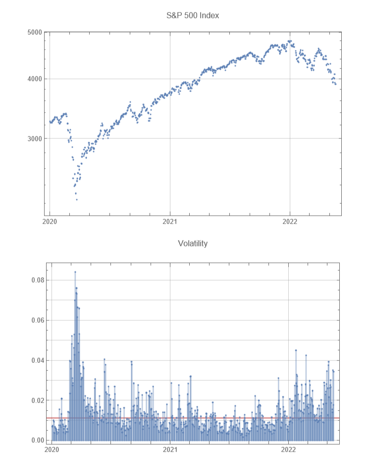
The current period shows a crash caused by lock downs to curtail the pandemic and the economic consequences. The graphs show that the point of maximum volatility occurs with the market bottom. There is concern that we are currently entering a bear market. So far there is no sign that the current decline has reached a bottom coinciding with a very sharp spike in volatility followed by declining volatility. The red line on the volatility graph represents the median volatility for the graph.
In[]:=
period=covid;median=Median[Log[#2[[2]]/#2[[3]]]&@@@period];max=Max[Log[#2[[2]]/#2[[3]]]&@@@period];GraphicsColumn[{DateListLogPlot[{#1,#2[[4]]}&@@@period,Joined->False,GridLines->Automatic,ImageSize->Large,PlotLabel->"S&P 500 Index"],DateListPlot[{{#1,Log[#2[[2]]/#2[[3]]]}&@@@period},Joined->False,Filling->Axis,FillingStyleDirective[Opacity[0.4],Thick],GridLines{Automatic,{Sequence@@Table[i,{i,0,Ceiling[max,0.01],0.01}],{median,Directive[Darker[Red],Thick]}}},PlotRange->All,ImageSize->Large,PlotLabel->"Volatility"]}]
Out[]=
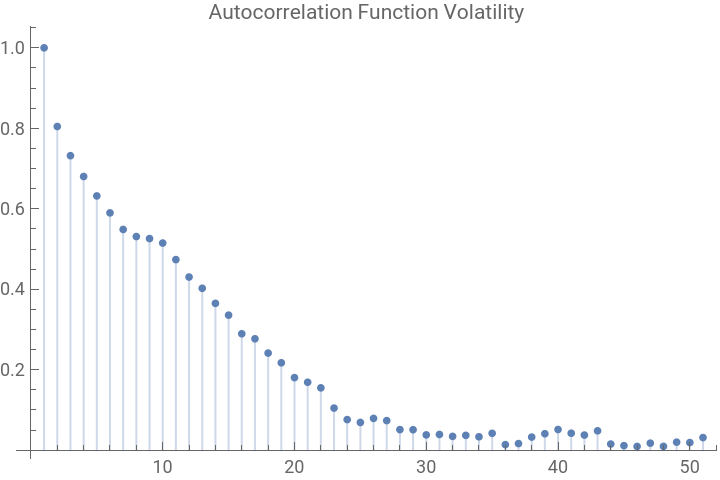
Here is some analysis of the volatility measure for the above period. There is strong serial dependence in the data as shown by the autocorrelation function.
In[]:=
vol=Log[#2[[2]]/#2[[3]]]&@@@covid;ListPlot[CorrelationFunction[vol,{50}],Filling->0,PlotRangeAll,PlotLabel->"Autocorrelation Function Volatility"]
Out[]=
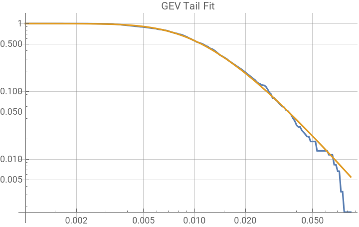
Despite the serial dependence the data are well fit by a Fréchet type of extreme value distribution.
In[]:=
edf=EmpiricalDistribution[vol];gev=EstimatedDistribution[vol,MaxStableDistribution[μ,σ,ξ]]
Out[]=
MaxStableDistribution[0.00891461,0.00529365,0.337855]
In[]:=
LogLogPlot[{1-CDF[edf,x],1-CDF[gev,x]},{x,0.001,Max[vol]},PlotRangeAll,GridLines->Automatic,PerformanceGoal"Speed",PlotLabel"GEV Tail Fit"]
Out[]=
In[]:=
HTgev=DistributionFitTest[vol,gev,"HypothesisTestData"];HTgev["TestDataTable",All]
Out[]=
Statistic | P-Value | |
Anderson-Darling | 0.443232 | 0.804961 |
Cramér-von Mises | 0.0457885 | 0.901311 |
Kolmogorov-Smirnov | 0.0225483 | 0.912595 |
Kuiper | 0.0399769 | 0.777387 |
Pearson 2 χ | 19.0631 | 0.794084 |
Watson 2 U | 0.043167 | 0.788322 |
The power tail exponent is close to 3.0 which is typical for the S&P 500 log return tail behavior.
In[]:=
1/gev[[3]]
Out[]=
2.95985
In[]:=
Median[vol]Median[gev]
Out[]=
0.0111896
Out[]=
0.01098
This compares the estimated and empirical density curves.
In[]:=
skd=SmoothKernelDistribution[vol];Plot[{PDF[skd,x],PDF[gev,x]},{x,Min[vol],Max[vol]},PlotLegends->{"Empirical Density","GEV Fit Density"}]
Out[]=


2008 Market Crash
2008 Market Crash
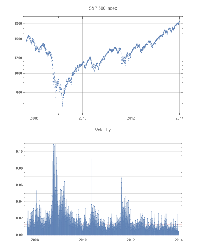
For this market crash the peak volatility occurred at a local minimum that preceded the slightly later final market bottom.
Out[]=
2000 Market Crash
2000 Market Crash
This market crash had three local minima and the peak volatility was nearest the second. The market recovery gained momentum as volatility decreased.
1987 Market Crash
1987 Market Crash
Here there was one very extreme volatility spike on October 19. The bottom was tested again a few days later.
1974 Market Crash
1974 Market Crash
Here again, the market bottom coincided with a peak volatility spike. The graph also shows an earlier market decline in 1970 with the bottom occurring near the peak volatility.