Liquid Liquid Equilibrium Using NDSolve
Case of a ternary system: water - ethyl acetate - acetone at 15 °C
Authors: Housam Binous and Ahmed Bellagi
Liquid Liquid Equilibrium Using NDSolve
Case of a ternary system: water - ethyl acetate - acetone at 15 °C
Authors: Housam Binous and Ahmed Bellagi
Case of a ternary system: water - ethyl acetate - acetone at 15 °C
Authors: Housam Binous and Ahmed Bellagi
We show how one can solve a system of nonlinear algebraic equations using NDSolve . The solution to the algebraic equations is indeed the steady state solution of a system of ODEs . This method is successfully applied to compute a tie line for the case of water - ethyl acetate - acetone at 15 °C .
In[]:=
Off[General::"spell1"]
water = component 1
ethyl acetate = component 2
acetone = component 3
Activities using the NRTL model
ethyl acetate = component 2
acetone = component 3
Activities using the NRTL model
In[]:=
GAMMA1=Exp[(t21/(RT)G21x2+t31/(RT)G31x3)/(x1+G21x2+G31x3)+x1/(x1+G21x2+G31x3)(-(x2t21/(RT)G21+x3t31/(RT)G31)/(x1+G21x2+G31x3))+x2G12/(G12x1+x2+G32x3)(t12/(RT)-(x1t12/(RT)G12+x3t32/(RT)G32)/(G12x1+x2+G32x3))+x3G13/(G13x1+G23x2+x3)(t13/(RT)-(x1t13/(RT)G13+x2t23/(RT)G23)/(G13x1+G23x2+x3))]
Out[]=
x1--
G21t21x2
RT
G31t31x3
RT
2
(x1+G21x2+G31x3)
G21t21x2
RT
G31t31x3
RT
x1+G21x2+G31x3
G13x3-+
t13
RT
G13t13x1
RT
G23t23x2
RT
G13x1+G23x2+x3
G13x1+G23x2+x3
G12x2-+
t12
RT
G12t12x1
RT
G32t32x3
RT
G12x1+x2+G32x3
G12x1+x2+G32x3
In[]:=
GAMMA1p=Exp[(t21/(RT)G21xp2+t31/(RT)G31xp3)/(xp1+G21xp2+G31xp3)+xp1/(xp1+G21xp2+G31xp3)(-(xp2t21/(RT)G21+xp3t31/(RT)G31)/(xp1+G21xp2+G31xp3))+xp2G12/(G12xp1+xp2+G32xp3)(t12/(RT)-(xp1t12/(RT)G12+xp3t32/(RT)G32)/(G12xp1+xp2+G32xp3))+xp3G13/(G13xp1+G23xp2+xp3)(t13/(RT)-(xp1t13/(RT)G13+xp2t23/(RT)G23)/(G13xp1+G23xp2+xp3))]
Out[]=
xp1--
G21t21xp2
RT
G31t31xp3
RT
2
(xp1+G21xp2+G31xp3)
G21t21xp2
RT
G31t31xp3
RT
xp1+G21xp2+G31xp3
G13xp3-+
t13
RT
G13t13xp1
RT
G23t23xp2
RT
G13xp1+G23xp2+xp3
G13xp1+G23xp2+xp3
G12xp2-+
t12
RT
G12t12xp1
RT
G32t32xp3
RT
G12xp1+xp2+G32xp3
G12xp1+xp2+G32xp3
In[]:=
GAMMA2=Exp[(t12/(RT)G12x1+t32/(RT)G32x3)/(G12x1+x2+G32x3)+x1G21/(x1+G21x2+G31x3)(t21/(RT)-(x2t21/(RT)G21+x3t31/(RT)G31)/(x1+G21x2+G31x3))+x2/(G12x1+x2+G32x3)(-(x1t12/(RT)G12+x3t32/(RT)G32)/(G12x1+x2+G32x3))+x3G23/(G13x1+G23x2+x3)(t23/(RT)-(x1t13/(RT)G13+x2t23/(RT)G23)/(G13x1+G23x2+x3))]
Out[]=
x2--
G12t12x1
RT
G32t32x3
RT
2
(G12x1+x2+G32x3)
G12t12x1
RT
G32t32x3
RT
G12x1+x2+G32x3
G23x3-+
t23
RT
G13t13x1
RT
G23t23x2
RT
G13x1+G23x2+x3
G13x1+G23x2+x3
G21x1-+
t21
RT
G21t21x2
RT
G31t31x3
RT
x1+G21x2+G31x3
x1+G21x2+G31x3
In[]:=
GAMMA2p=Exp[(t12/(RT)G12xp1+t32/(RT)G32xp3)/(G12xp1+xp2+G32xp3)+xp1G21/(xp1+G21xp2+G31xp3)(t21/(RT)-(xp2t21/(RT)G21+xp3t31/(RT)G31)/(xp1+G21xp2+G31xp3))+xp2/(G12xp1+xp2+G32xp3)(-(xp1t12/(RT)G12+xp3t32/(RT)G32)/(G12xp1+xp2+G32xp3))+xp3G23/(G13xp1+G23xp2+xp3)(t23/(RT)-(xp1t13/(RT)G13+xp2t23/(RT)G23)/(G13xp1+G23xp2+xp3))]
Out[]=
xp2--
G12t12xp1
RT
G32t32xp3
RT
2
(G12xp1+xp2+G32xp3)
G12t12xp1
RT
G32t32xp3
RT
G12xp1+xp2+G32xp3
G23xp3-+
t23
RT
G13t13xp1
RT
G23t23xp2
RT
G13xp1+G23xp2+xp3
G13xp1+G23xp2+xp3
G21xp1-+
t21
RT
G21t21xp2
RT
G31t31xp3
RT
xp1+G21xp2+G31xp3
xp1+G21xp2+G31xp3
In[]:=
GAMMA3=Exp[(t13/(RT)G13x1+t23/(RT)G23x2)/(G13x1+G23x2+x3)+x1G31/(x1+G21x2+G31x3)(t31/(RT)-(x2t21/(RT)G21+x3t31/(RT)G31)/(x1+G21x2+G31x3))+x2G32/(G12x1+x2+G32x3)(t32/(RT)-(x1t12/(RT)G12+x3t32/(RT)G32)/(G12x1+x2+G32x3))+x3/(G13x1+G23x2+x3)(-(x1t13/(RT)G13+x2t23/(RT)G23)/(G13x1+G23x2+x3))]
Out[]=
--x3
G13t13x1
RT
G23t23x2
RT
2
(G13x1+G23x2+x3)
G13t13x1
RT
G23t23x2
RT
G13x1+G23x2+x3
G31x1-+
t31
RT
G21t21x2
RT
G31t31x3
RT
x1+G21x2+G31x3
x1+G21x2+G31x3
G32x2-+
t32
RT
G12t12x1
RT
G32t32x3
RT
G12x1+x2+G32x3
G12x1+x2+G32x3
In[]:=
GAMMA3p=Exp[(t13/(RT)G13xp1+t23/(RT)G23xp2)/(G13xp1+G23xp2+xp3)+xp1G31/(xp1+G21xp2+G31xp3)(t31/(RT)-(xp2t21/(RT)G21+xp3t31/(RT)G31)/(xp1+G21xp2+G31xp3))+xp2G32/(G12xp1+xp2+G32xp3)(t32/(RT)-(xp1t12/(RT)G12+xp3t32/(RT)G32)/(G12xp1+xp2+G32xp3))+xp3/(G13xp1+G23xp2+xp3)(-(xp1t13/(RT)G13+xp2t23/(RT)G23)/(G13xp1+G23xp2+xp3))]
Out[]=
--xp3
G13t13xp1
RT
G23t23xp2
RT
2
(G13xp1+G23xp2+xp3)
G13t13xp1
RT
G23t23xp2
RT
G13xp1+G23xp2+xp3
G31xp1-+
t31
RT
G21t21xp2
RT
G31t31xp3
RT
xp1+G21xp2+G31xp3
xp1+G21xp2+G31xp3
G32xp2-+
t32
RT
G12t12xp1
RT
G32t32xp3
RT
G12xp1+xp2+G32xp3
G12xp1+xp2+G32xp3
In[]:=
G12=Exp[-a12t12/(RT)];G21=Exp[-a12t21/(RT)];G13=Exp[-a13t13/(RT)];G31=Exp[-a13t31/(RT)];G32=Exp[-a32t32/(RT)];G23=Exp[-a32t23/(RT)];
Gas constant, temperature and binary interaction parameters for the NRTL model
In[]:=
R=1.987;a13=0.585600018501282;a12=0.410400003194809;a32=0.291200011968613;t31=750.318115234375;t13=1299.39501953125;t23=467.125701904297;t32=-304.988403320313;t12=2316.36303710938;t21=935.687927246094;
T=273.15+15(*inKelvin*)
Out[]=
288.15
Computing a Tie line with FindRoot
In[]:=
X1=0.7;X2=0.2;
In[]:=
sol[1]=FindRoot[{(GAMMA1x1GAMMA1pxp1),(GAMMA2x2GAMMA2pxp2),(GAMMA3x3GAMMA3pxp3),(x1L+xp1LpX1),(x2L+xp2LpX2),(1xp1+xp2+xp3),(1x1+x2+x3),(L+Lp1)},{x1,0.95},{x2,0.01},{xp1,0.5},{xp2,0.4},{L,0.05},{Lp,0.04},{x3,0.01},{xp3,0.1}, MaxIterations10000]
Out[]=
{x10.966869,x20.0123889,xp10.574088,xp20.288517,L0.320566,Lp0.679434,x30.0207426,xp30.137395}
Computing a Tie line with NDSolve
Coordinates of the first point on the tie line.
In[]:=
x1=sol[1][[1,2]]
Out[]=
0.966869
In[]:=
x2=sol[1][[2,2]]
Out[]=
0.0123889
In[]:=
x3=1-x1-x2
Out[]=
0.0207426
Using NDSolve to look for the steady state, which corresponds to the solution of the nonlinear algebraic equations.
In[]:=
sol1=NDSolve[{D[xp1[t],{t,1}](GAMMA1x1-GAMMA1pxp1/.xp1xp1[t]/.xp2xp2[t]/.xp3xp3[t]),D[xp2[t],{t,1}](GAMMA2x2-GAMMA2pxp2/.xp1xp1[t]/.xp2xp2[t]/.xp3xp3[t]),D[xp3[t],{t,1}](GAMMA3x3-GAMMA3pxp3/.xp1xp1[t]/.xp2xp2[t]/.xp3xp3[t]),xp1[0]0.4,xp2[0]0.2,xp3[0]0.1},{xp1,xp2,xp3},{t,0,1000}]
Out[]=
xp1InterpolatingFunction,xp2InterpolatingFunction,xp3InterpolatingFunction


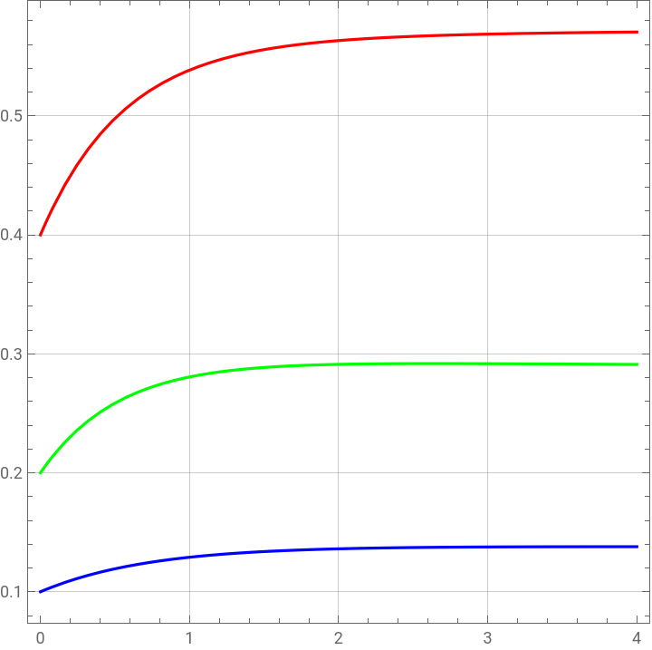
Coordinates of the second point on the tie line are the steady state solution (obtained at t=1000). We get the same result as the one found using FindRoot (xp1, xp2, xp3)
In[]:=
First[Evaluate[xp1[t]/.sol1/.t1000]]
Out[]=
0.574088
In[]:=
First[Evaluate[xp2[t]/.sol1/.t1000]]
Out[]=
0.288517
In[]:=
First[Evaluate[xp3[t]/.sol1/.t1000]]
Out[]=
0.137395
We reach the steady state rapidly (we are almost at the steady state at t=4).
In[]:=
Plot[{Evaluate[xp1[t]/.sol1],Evaluate[xp2[t]/.sol1],Evaluate[xp3[t]/.sol1]},{t,0,4},PlotStyle{RGBColor[1,0,0],RGBColor[0,1,0],RGBColor[0,0,1]},Frame->True,GridLines->Automatic,AspectRatio->1,PlotLegends->LineLegend[{RGBColor[1,0,0],RGBColor[0,1,0],RGBColor[0,0,1]},{"water","ethylacetate","acetone"}]]
Out[]=