If some parts of our universe have fractional dimensions, it will be necessary to have solutions for electromagnetic fields which are valid in such regions. When we represent our universe through hypergraphs, the possibility of a universe with a fractional dimension is high. In this project, we will try to explore such a possibility and then find the fields due to some simple configurations like a point charge or a dipole. One approach we can take is to find the solutions of Maxwell’s equations in the general D (integral) dimension and use analytic continuation to find solutions for the fractional case. The other possibility could be to write the field equations in fractional dimensions and explore their solutions.
1. Introduction
1. Introduction
Wolfram Physics Project has tried to set up a class of models that are simple and structureless but can still provide a foundation from which various complex physical phenomena can emerge. The idea of Quantum Mechanics, Relativity, and General relativity emerge from some classes of models. However,electromagnetism is not yet captured nicely in the picture. But, if history is to mean something, electromagnetism always played a leading role in the formulation of theories. Despite the ubiquitous influence of gravity in real day-to-day life, it was electromagnetism for which a proper field theory was first formulated by James Clerk Maxwell in 1965 where electricity, magnetism, and light are shown to be a different manifestations of the same phenomenon. This has been called the second great unification in physics after Newton’s work. This field theoretic unification ushered in the era of modern physics. Einstein’s relativity came directly from the incompatibility of Maxwell’s theory with Galilean relativity. Einstein’s desire to make a similar field theory for gravity led to General relativity. The UV catastrophe in the classical picture of the black body spectrum forced Physicists to develop Quantum theory. Even in the 20th century, Quantum Electrodynamics is the first quantum field theory that successfully combined special relativity and quantum mechanics. Richard Feynman has called quantum electrodynamics the “jewel of physics” for its extremely accurate predictions. Given this history, it is of utmost importance that we develop a proper framework within the Wolfram Physics Project where electromagnetism exists naturally. That is the ultimate goal of a series of projects like this. In this project, we consider a particularly smaller aspect of that. As we will see below, in Wolfram’s models the dimension of space can be fractional. Here we will consider how we can generalize Maxwell’s theory in such fractional dimensional space. In particular, we will take Poisson’s equation and solve it for simple configurations like Point charge and electric dipole. In section 2, we will give a summary of the theory and calculations on how to calculate electric potential on fractional dimensional space. We will see two approaches: the first one is to find the potential in an integral dimensional space and analytically continue to fractional dimensional space. The second approach is to assume the fractional nature of space from the beginning and calculate the potential. We will show that these two approaches are equivalent. In section 3, we will discuss how fractional dimensional space arises in Wolfram Models. In section 4, some phenomenological aspects of this are discussed using Wolfram language, finally, in section 5, we give our conclusions and prospects for future work. The appendix with the detailed codes follows the conclusion.
2. Theory and Calculations
2. Theory and Calculations
Lets begin our consideration with the Maxwell’s equations:∇·E = (Gauss law of electricity)∇·B = 0 (Gauss law of magnetism)∇ × E = (Faraday’s law of induction)∇ × B = (J+ ) (Faraday’s law of induction)
ρ
ϵ
0
-
∂B
∂t
μ
0
ϵ
0
∂E
∂t
Method 1: Finding solution in General D dimension and continuing analytically
Method 1: Finding solution in General D dimension and continuing analytically
We consider a single point charge, q, at the origin and find the electric field strength at a distance r from the origin. Taking the first Gauss’ law in D-dimension and using divergence theorem we obtain:
E(r)
Γ(D/2)
2
D/2
π
ϵ
0
q
D-1
r
Lets first visualize this field and compare the fractional case with integral case around D=3.
In[]:=
electricField[r_,d_]:=*
Gamma[d/2]
2*
d/2
π
1
d-1
r
In[]:=
Manipulate[Plot[{electricField[r,3],electricField[r,d]},{r,0,10},PlotStyle{Red,Blue},PlotLegendsPlaced[{"D = 3",StringJoin["D = ",ToString[d]]},{0.7,0.7}],PlotTheme"Scientific",FrameLabel->{Style["r",15],Style["E(r)",15]},PlotLabel"The Electric Field Strength for D Dimensions"],{d,2.1,3.0,0.05}]
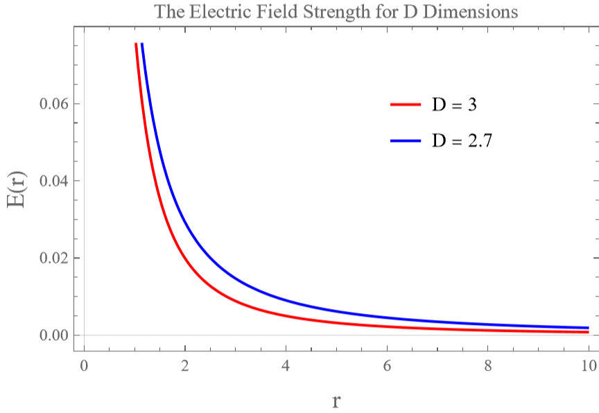
From this electric field strength, we can easily obtain the potential,
ϕ(r)
Γ(D/2-1)
4
D/2
π
ϵ
0
q
D-2
r
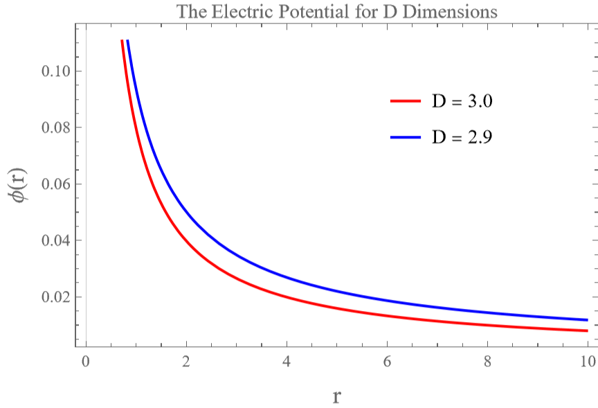
We then visualize the potential:
In[]:=
electricPotential[r_,d_]:=*
Gamma[(d/2)-1]
4*
d/2
π
1
d-2
r
In[]:=
Manipulate[Plot[{electricPotential[r,3],electricPotential[r,d]},{r,0,10},PlotStyle{Red,Blue},PlotLegendsPlaced[{"D = 3.0",StringJoin["D = ",ToString[d]]},{0.7,0.7}],PlotTheme"Scientific",FrameLabel->{Style["r",15],Style["ϕ(r)",15]},PlotLabel"The Electric Potential for D Dimensions"],{d,2.1,3,0.05}]
Method 2: Taking Poisson’s Equation for Fractional Case
Method 2: Taking Poisson’s Equation for Fractional Case
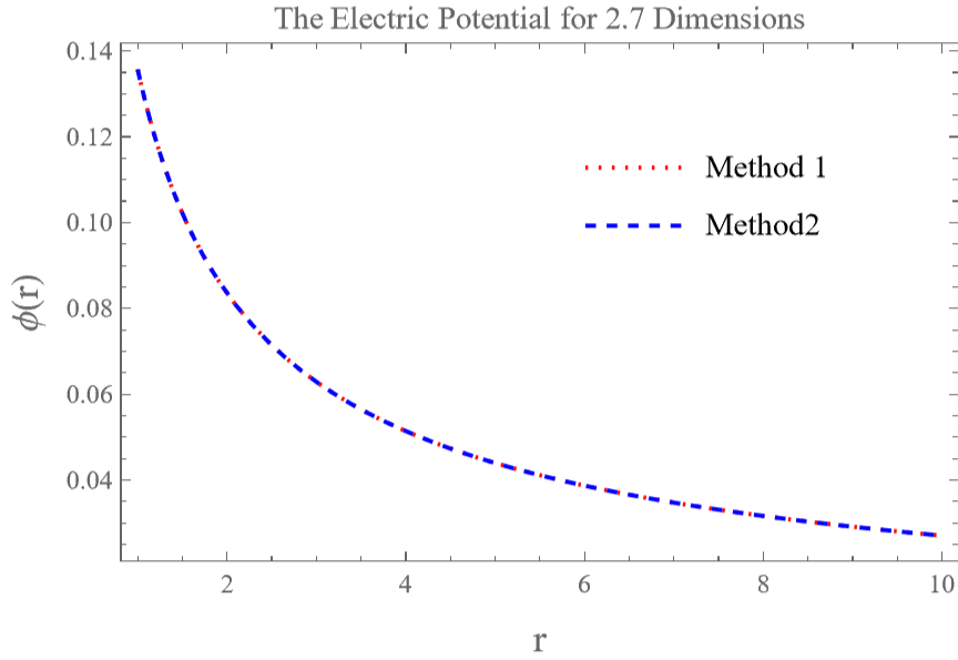
The other method would be to take the Poisson’s equations in D=2+α dimension, where 0<α<1, and solve for the potential due to a point charge. The Poisson’s equation for a point charge source:ϕ = -(r)Because D = 2+α with α non-integer, we will use Mandelbrot scaling in the integration:x = xdxWith the use of this scaling, one can prove that the various ordinary properties of Dirac-Delta function and the Fourier transform are valid for the fractional dimensional case as well. Then taking fourier transform of the Poisson’s equation, one reaches at the following solution for the potential.We would then like to compare this result with the first method. The following code will take few minutes to run:
2
∇
q
ϵ
0
D
δ
α
d
α/2
π
α-1
|
Γ(α/2)
ϕ(r)(ρr)dρ
q
ϵ
0
1+α/2
(2π)
1
α/2
r
∞
∫
0
J
α/2
1-α/2
ρ
In[]:=
electricPotential2[r_,alpha_]:=NIntegrate,{rho,0,Infinity}
1
1+alpha/2
(2Pi)
alpha/2
r
BesselJ[alpha/2,rho*r]
1-alpha/2
rho
In[]:=
Plot[{electricPotential[r,2.7],electricPotential2[r,0.7]},{r,1,10},PlotStyle{{Red,Dotted},{Blue,Dashed}},PlotLegendsPlaced[{"Method 1","Method2"},{0.7,0.7}],PlotTheme"Scientific",FrameLabel->{Style["r",15],Style["ϕ(r)",15]},PlotLabel"The Electric Potential for 2.7 Dimensions"]
In[]:=
Plot[{electricPotential[r,2.9],electricPotential2[r,0.9]},{r,1,10},PlotStyle{{Red,Dotted},{Blue,Dashed}},PlotLegendsPlaced[{"Method 1","Method2"},{0.7,0.7}],PlotTheme"Scientific",FrameLabel->{Style["r",15],Style["ϕ(r)",15]},PlotLabel"The Electric Potential for 2.9 Dimensions"]
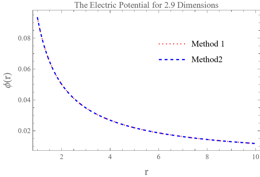
The above plots clearly show the equivalence of two approaches considered above. Therefore, in what follows we won’t distinguish between these two methods and use the method 1 which is faster to implement. The bottom line is that our results for integral D-dimension can be analytically continued to cases where D could be fractional.
3. Fractional Dimensional Space in Wolfram Models
3. Fractional Dimensional Space in Wolfram Models
In Wolfram Model, we begin with some simple replacement rules and apply them iteratively, just like in the Koch Curve. Lets take the following example from Wolfram Physics introductory textbook. The following is a replacement rule:
If we use this replacement rule and run our model for 500 iterations, a nice structure starts to emerge:
The dimension of the plot goes to 2 as we take reasonably larger values of r. By “reasonably”, we mean that the value of r is still small as compared to the whole graph so as to avoid the boundary effects. This definition of dimension and the Hausdorff dimension look different but are similar. In what follows, we will take them to be the same, which they are in a restricted sense.
Simple Construction of a Fractional Dimensional Space
Simple Construction of a Fractional Dimensional Space
We consider a simple two dimensional grid as shown below. We will call such grid “Without Additional Edges”, a name that will make sense after we see the next diagram.
We can add edges to such a grid to change the dimension. As an example, we could add diagonal edges from left bottom to right top in each cell. We will call such a diagram “With 1-Diagonal Edges”.
Similarly, we can add another diagonal from right bottom to left top in each cell. We will call such diagram “With 2-Diagonal Edges”.
In order to see how dimension changes when we add edges in these manners, we take a large grid (51 x 51) and compare their dimensions before and after adding edges. The dimensions are calculated about the center of the grid. We have terminated the calculation of dimension as we got closer to the boundary.
Note: Before running the following code, please run Section 1 of the appendix.
Note: Before running the following code, please run Section 1 of the appendix.
Similarly, we can consider 3D grid and add edges.
To see how the dimension changes, we consider a (25x25x25) grid.
Note: Before running the following code, please run Section 2 of the appendix.
Note: Before running the following code, please run Section 2 of the appendix.
As we had expected, we see that with addition of edges, the dimension of the grid goes up a little. By adding such edges, we can take an integer dimension space and construct fractional dimensional space from it using Wolfram Language. In the next section, we will also consider other ways of making fractional space.
4. Phenomenology
4. Phenomenology
In section 2, we saw how to calculate electric potential due to a point charge in any types of space. In section 3, we considered how fractional dimensional space arises in Wolfram model and also a simple way to construct one from a 2D grid or a 3D grid. In the section, we will combine these two results. It will be difficult to visualize the differences if we considered the 3D grid because the 2D representation will be too crowded with dots and lines. Therefore, we will consider the 2D grid and see how the equipotential surfaces varies among these constructions and also make a sanity check of whether it makes sense.
Equipotential Surface due to a Point Charge in 2D Grids
Equipotential Surface due to a Point Charge in 2D Grids
Note : Please run Section 3 in the Appendix before running the following code. This might take several minutes.
Although the vertex size and colors are exact in the above image, the image is not very clear to see. In particular, we cannot see clearly what the shape of potential surfaces are. So we will enhance its colors slightly in the following image. The size of the vertices still correspond to the electric potential.
Note: Please run Section 4 in the Appendix before running the following code.
Note: Please run Section 4 in the Appendix before running the following code.
To further see the equipotential surfaces clearly, we will enhance both its vertex weight and its color slightly in the following image.
Note : Please run Section 5 in the Appendix before running the following code .
Note : Please run Section 5 in the Appendix before running the following code .
We see that the shape of the equipotential surface changes depending on the geometry we are using. We also see that further we go, the potential gets smaller as seen by the red shift or smaller sizes of the vertex. One crucial point can be seen from the first plot in this section. We see that even at the same distance from the center, the potential is smaller for the second and third grid. That makes sense because the Hausdorff dimension of second and the third grid is larger so potential dies off quickly as compared to the first grid.
Equipotential Surface due to a Physical Dipole in a 2D Grids
Equipotential Surface due to a Physical Dipole in a 2D Grids
A very similar approach can be taken to consider equipotential surfaces due to a physical dipole. We consider a physical dipole: two opposite point charges kept at a finite distance from each other. We won’t consider an ideal dipole because the definition of potential will require some notion of angle which we haven’t defined here.
Note : Please run Section 6 in the Appendix before running the following code .
We see similar effects of dimension on the potential. Another interesting aspect of this is the shape of zero potential region. On the first grid, the zero potential region is a line lying in between the two charges. On the second grid, it is a shape of triangle on either side of the charges, in a diagonal sense. On the third grid, its a triangle again but isosceles in this case.
Equipotential Surfaces using a Sprinkling Graph
Equipotential Surfaces using a Sprinkling Graph
Note : Please run Section 7 in the Appendix before running the following code .
Equipotential Surfaces using a Graph Derived using a Rule
Equipotential Surfaces using a Graph Derived using a Rule
As a final example, we want to consider a rule:
We will iterate this rule 10 times and convert the hypergraph generated to undirected graph. The point at about the center of whole graph where a point charge is kept is colored black. The potential is then calculated at all the vertices and the vertices are colored and sized in accordance with the value of potential. The further from the charge you go, the lower is the potential.
Note : Please run Section 8 in the Appendix before running the following code .
Note : Please run Section 8 in the Appendix before running the following code .
5. Concluding remarks
5. Concluding remarks
6. Acknowledgment
6. Acknowledgment
First of all, I would like to thank my mentors Alessandro Pisani and Xerxes Arsiwalla for their feedback, suggestions and support, and Stephen Wolfram for suggesting this project to me and his comments. I would also like to thank Jonthan Gorard and David Chester for their comments and suggestions. I must also thank Utkarsh Bajaj, Simone Fischer and Swastik Banerjee for useful discussions. And, finally, I would like to thank all the participants in the Wolfram Summer School 2022 along with staff who made this journey fun.
7. References
7. References
◼
S I Muslih and O P Agrawal, Fractional Dynamics and Control, (Springer, New York, 2010), 217
◼
B Zwiebach, A First Course in String Theory, (Cambridge University Press, UK, 2004), 40
Appendix
Appendix
The detail codes are given here. In order to run all of the notebook, one must run these codes too. We have left smaller codes within the text and only copied larger codes in this section. We have also indicated in the main text so as to which subsection of codes in this appendix should be run before running the corresponding codes in the text.
Section 1: Comparison of Hausdorff Dimension for 2D Grid
Section 1: Comparison of Hausdorff Dimension for 2D Grid
Note: The following code will take about a minute to run.
Section 2: Comparison of Hausdorff Dimension for 3D Grid
Section 2: Comparison of Hausdorff Dimension for 3D Grid
Note : The following code will take several minutes to run .
Section 3: Equipotential Surface with exact vertex weight and colors based on the potential at the point
Section 3: Equipotential Surface with exact vertex weight and colors based on the potential at the point
Note : The following code will take several minutes to run .
Section 4: Equipotential Surface with exact vertex weight but vertex colors enhanced for Aesthetic Purposes
Section 4: Equipotential Surface with exact vertex weight but vertex colors enhanced for Aesthetic Purposes
Section 5: Equipotential Surface with both vertex weight and colors enhanced for Aesthetic Purposes
Section 5: Equipotential Surface with both vertex weight and colors enhanced for Aesthetic Purposes
Section 6: Equipotential Surface for a Physical Dipole with exact vertex weight and colors
Section 6: Equipotential Surface for a Physical Dipole with exact vertex weight and colors
Section 7: Equipotential Surfaces using a Sprinkling Graph
Section 7: Equipotential Surfaces using a Sprinkling Graph
Section 8: Equipotential Surfaces using a Graph derived from a Rule
Section 8: Equipotential Surfaces using a Graph derived from a Rule