ABSTRACT (original article): The Gray configuration is a configuration which typically is realized as the points and lines of the 3 x 3 x 3 integer lattice. It occurs as a member of an infinite family of configurations defined by Bouwer in 1972. Since their discovery, both the Gray configuration and its Levi graph (i.e., its point-line incidence graph) have been the subject of intensive study. Its automorphism group contains cyclic subgroups isomorphic to and , so it is natural to ask whether the Gray configuration can be realized in the plane with any of the corresponding rotational symmetry. In this paper, we show that there are two distinct polycyclic realizations with symmetry. In contrast, the only geometric polycyclic realization with straight lines and symmetry is only a “weak” realization, with extra unwanted incidences (in particular, the realization is actually a configuration). CITATION (original article): Leah Wrenn Berman, Gábor Gévay, Tomaž Pisanski, Polycyclic Geometric Realizations of the Gray Configuration, arXiv:2502.14484. https://doi.org/10.48550/arXiv.2502.14484
()
27
3
3
9
3
9
()
27
4
A configuration of points and lines is a collection of points and n lines in which each point lies on k lines and each line passes through points.
()
n
k
n
k
The Gray Graph is a bipartite cubic graph on 54 vertices that is edge-transitive but not vertex-transitive. If the bipartition of the vertices of the graph are associated with geometric points and straight lines, with two vertices in the graph being adjacent if and only if the corresponding points and lines are incident geometrically, the Gray graph is the incidence structure of a configuration, which can be realized as the points and segments of the integer lattice.
()
27
3
3x3x3
In[]:=
cfgPts=Flatten[Table[{i,j,k},{i,0,2},{j,0,2},{k,0,2}],2]Length[cfgPts]
Out[]=
{{0,0,0},{0,0,1},{0,0,2},{0,1,0},{0,1,1},{0,1,2},{0,2,0},{0,2,1},{0,2,2},{1,0,0},{1,0,1},{1,0,2},{1,1,0},{1,1,1},{1,1,2},{1,2,0},{1,2,1},{1,2,2},{2,0,0},{2,0,1},{2,0,2},{2,1,0},{2,1,1},{2,1,2},{2,2,0},{2,2,1},{2,2,2}}
Out[]=
27
In[]:=
cfgLines=Join[Flatten[Table[{{i,0,k},{i,2,k}},{i,0,2},{k,0,2}],1],Flatten[Table[{{i,k,0},{i,k,2}},{i,0,2},{k,0,2}],1],Flatten[Table[{{0,i,k},{2,i,k}},{i,0,2},{k,0,2}],1]]Length[cfgLines]
Out[]=
{{{0,0,0},{0,2,0}},{{0,0,1},{0,2,1}},{{0,0,2},{0,2,2}},{{1,0,0},{1,2,0}},{{1,0,1},{1,2,1}},{{1,0,2},{1,2,2}},{{2,0,0},{2,2,0}},{{2,0,1},{2,2,1}},{{2,0,2},{2,2,2}},{{0,0,0},{0,0,2}},{{0,1,0},{0,1,2}},{{0,2,0},{0,2,2}},{{1,0,0},{1,0,2}},{{1,1,0},{1,1,2}},{{1,2,0},{1,2,2}},{{2,0,0},{2,0,2}},{{2,1,0},{2,1,2}},{{2,2,0},{2,2,2}},{{0,0,0},{2,0,0}},{{0,0,1},{2,0,1}},{{0,0,2},{2,0,2}},{{0,1,0},{2,1,0}},{{0,1,1},{2,1,1}},{{0,1,2},{2,1,2}},{{0,2,0},{2,2,0}},{{0,2,1},{2,2,1}},{{0,2,2},{2,2,2}}}
Out[]=
27
In[]:=
Graphics3D[{AbsolutePointSize[6],Red,Point[cfgPts],Blue,Line[cfgLines]},Method->{"ShrinkWrap"->True},Boxed->False]
Out[]=

In the article “Polycyclic Geometric Realizations of the Gray Configuration”, published in the Australasian Journal of Combinatorics, https://ajc.maths.uq.edu.au, Leah Wrenn Berman, Gábor Gévay and Tomaž Pisanski considered ways of drawing the Gray Configuration that are “polycyclic”, meaning that it can be realized using rotational symmetry, so that the points and lines are partitioned into orbits in which each orbit has the same number of points. (In the above drawing of the Gray configuration, the realization has rotational symmetry in 3-space, but any of the isometries of the configuration have some points that are fixed, and some that are not, so that the orbits under the maximal rotational symmetry group do not all have the same size.
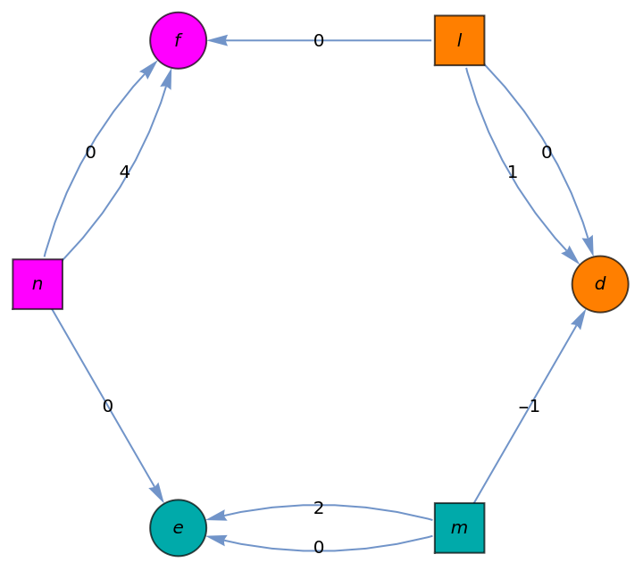
Through various analyses in the paper, it is shown that one of the possible ways to attempt to realize the Gray configuration in a polycyclic fashion is with 9-fold rotational symmetry. If such a realization were possible, then the configuration would have three symmetry classes of points, which could be labeled D, E, F, and three symmetry classes of lines, labeled L, M ,N, which would need to have a voltage graph (an edge-labeled digraph which corresponds to a quotient of the realization under the Z_9 symmetry group) with voltage group Z_9 of the following form:
(*usinglowercasetoavoidspecialmathematicaassignments*)Graph{d,l,f,n,e,m},{DirectedEdge[l,d,0],DirectedEdge[l,d,1],DirectedEdge[l,f,0],DirectedEdge[n,f,0],DirectedEdge[n,f,4],DirectedEdge[n,e,0],DirectedEdge[m,e,0],DirectedEdge[m,e,2],DirectedEdge[m,d,-1]},
Out[]=
Geometric techniques exist to determine if a Z_m voltage graph of this form can be realized. Specifically, to construct a realization, we need to be able to do the following (with index arithmetic modulo 9):
1
.Construct points , as the vertices of a regular 9-gon; specifically, let =(cos(2πi/9),sin(2πi/9)).
D
i
i=0,1,...,8
D
i
2
.Construct lines =.
L
i
D
i
D
i+1
3
.Place a point (t) arbitrarily (parameterized by t) on line and let (t) be the rotation of through 2πi/9 about the origin.
F
0
L
0
F
i
F
0
4
.Construct lines (t)=(t)(t).
N
i
F
i
F
i+4
5
.Construct a circle C through the three points , and the origin.
D
-1
D
−1−2
6
.Construct point to be the intersection of line (t)with C, if it exists. If no point of intersection exists, then the algorithm fails. If a point of intersection exists, let be the rotation of through 2π i/9 about the origin.
E
0
N
0
E
i
E
0
7
.Construct lines =. The line will pass through the point .
M
i
E
i
E
i+2
M
i
D
i-1
It turns out that when we try to do this construction, most of the time, the line N_0(t) does not intersect the circle, and in fact, the only points of intersection are points of tangency. Specifically, we prove:
Theorem 7.2: There are exactly two positions of (t) on so that the line (t)=(t)(t) intersects the circle passing through the three points , and O. These two positions are precisely the points =∩ and =∩, and at these positions, the line (t)is tangent to . For all other values of t, the line (t) does not intersect . Therefore, any straight-line realization of the Gray Configuration with symmetry is a weak realization, because there are extra incidences caused by the fact that lies on two lines (rather than only one).
F
0
L
0
N
0
F
0
F
4
D
-1
D
-3
P
1
L
0
L
-3
P
2
L
0
L
3
N
0
N
0
9
F
0
L
i
This will be verified by computations in Mathematica, below. We will use the following lemma:
Lemma 7.3. Let ℓ be a line and let ℓ′ be the image of ℓ under rotation through some angle θ about a point O. Let P be an arbitrary point on ℓ and P′ the image of P under rotation through θ about O o f P (thus P′ lies on ℓ′). The envelope of the lines PP′ is a parabola with focus O and directrix formed by the line ,′, where , ′ are formed by reflecting O over ℓ, ℓ′ respectively.
O
ℓ
O
ℓ
O
ℓ
O
ℓ
Define the points as follows:
D
i
In[]:=
d[i_]:={Cos[2Pii/9+off],Sin[2Pii/9+off]}/.off->4*2Pi/9+Pi/18
We can look at the points, and the lines and .
L
0
L
4
In[]:=
Graphics[{AbsolutePointSize[6],Orange,Table[Point[d[i]],{i,0,9}],Table[Text[Subscript[D,i],d[i],{1,1}],{i,0,8}],InfiniteLine[{d[0],d[1]}],InfiniteLine[{d[4],d[5]}],Black,Point[{0,0}]}]
Out[]=
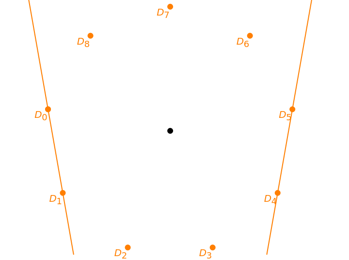
With this choice of coordinates, by Lemma 7.3, the lines and (which is the rotate of line through the angle about O), shown in Magenta, are tangent to a parabola P with focus at and axis of symmetry on the y-axis. In this image, you can move the slider to vary t and observe that the line (t) remains tangent to a parabola.
L
0
L
4
L
0
θ=4·2π/9
O=(0,0)
N
0
In[]:=
Manipulate[ContourPlot[Evaluate[x^2==4p(p+y)/.{p->Cos[Pi/9]Cos[4Pi/9]}],{x,-1.5,1.5},{y,-1.5,1.5},Epilog->{AbsolutePointSize[6],Orange,Table[Point[d[i]],{i,0,9}],Table[Text[Subscript[D,i],d[i],{1,1}],{i,0,8}],InfiniteLine[{d[0],d[1]}],InfiniteLine[{d[4],d[5]}],Black,Point[{0,0}],Magenta,InfiniteLine[{d[0],d[4]}],InfiniteLine[{d[1],d[5]}],Dashed,InfiniteLine[{(1-t)d[0]+(t)d[1],(1-t)d[4]+(t)d[5]}],Point[(1-t)d[0]+(t)d[1]],Text[Subscript[F,0],(1-t)d[0]+(t)d[1],{1,1}],Point[(1-t)d[4]+(t)d[5]],Text[Subscript[F,4],(1-t)d[4]+(t)d[5],{1,1}]}],{{t,-.5},-3,3},SaveDefinitions->True]
Out[]=


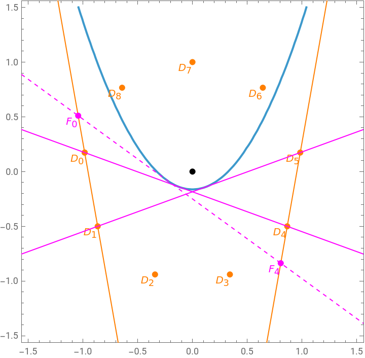
Similarly, we reflect the origin over line L_4 = D_4D_5.
Observe that these two points have the same y-coordinate, so the directrix is horizontal. We can verify the trigonometry:
The general formula of a parabola that opens up, whose axis of symmetry is the y-axis, and whose focus is at the origin, is x^2 = 4p^2 + 4py, where p is half the distance from the focus to the directrix.
We use this fact to define the parabola.
We can naively try simply solving for the intersections. Notice we get two points of intersection, repeated twice.
We could ask Mathematica to compute this intersection, but it doesn’t handle trigonmetry that well. We can use elementary right triangle trigonometry to produce a much cleaner set of coordinates.
Let pt2 be the rotate of pt1 by 4*2 Pi/9. We can use more elementary trigonometry to get the coordinates precisely.
Shall we verify? Sure.
Finally, we claim that the points pt1, tanPt1, and pt2 are collinear. We do this by using a projective geometry technique and determinants.
Sure enough, the determinant of the three points is 0, so they are collinear. We verify with a picture. The gray lines mark angles of pi/18 to help with the trigonometry.
So while it is possible to satisfy Algorithm 7.1, the only values also lie on other orange lines, which means that in the final construction of the configuration, each point actually lies on 4 lines rather than three (so it is a “weak” realization only). We can look at the final realization.
Combinatorially, this realizes the Gray configuration with 9-fold rotational symmetry, but it has inescapable extra incidences.
CITE THIS NOTEBOOK
CITE THIS NOTEBOOK
Polycyclic geometric realizations of the Gray configuration
by Leah Wrenn Berman, Gábor Gévay, Tomaž Pisanski
Wolfram Community, STAFF PICKS, February 3, 2026
https://community.wolfram.com/groups/-/m/t/3633790
by Leah Wrenn Berman, Gábor Gévay, Tomaž Pisanski
Wolfram Community, STAFF PICKS, February 3, 2026
https://community.wolfram.com/groups/-/m/t/3633790