So far it has not been proven that
anything in mathematics is difficult.
Norbert a’Campo
anything in mathematics is difficult.
Norbert a’Campo
Source: Riemann’s Zeta Function. H.M. Edwards 1974.
J(x)
x=0
1
2
1
3
J(x)
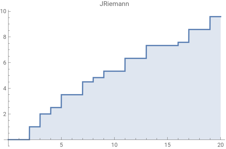
Riemann denotes the function by in his 1859 paper: “On the number of primes less than a given magnitude”.
J(x)
f(x)
In[]:=
JRiemann[x_]:=Sum[With[{fi=FactorInteger[n]},If[Length[fi]==1,1/Last[First[fi]],0]],{n,2,x}]
Example:
In[]:=
JRiemann[10]
Out[]=
16
3
In[]:=
Plot[JRiemann[x],{x,0,20},Filling->Axis,PlotLabel->"JRiemann"]
Out[]=
J(x)
π(x)
J(x)==
∞
∑
n=1
π()
1/n
x
n
log(2,x)
∑
n=1
π()
1/n
x
n
π()=0
1/n
x
1/n
x
In[]:=
QuietSolve==2,n
1/n
x
Out[]=
n
Log[x]
Log[2]
In[]:=
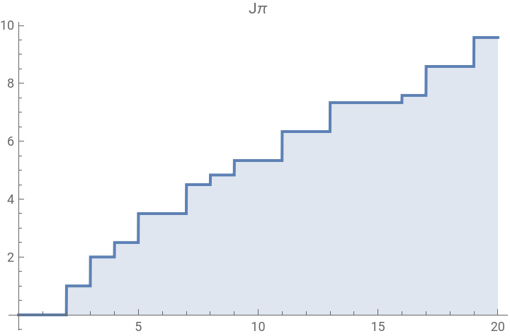
Jπ[x_]:=SumPrimePi[]n,{n,1,Log[2,x]}
1/n
x
Example :
In[]:=
Jπ[10]
Out[]=
16
3
In[]:=
Plot[Jπ[x],{x,0,20},Filling->Axis,PlotLabel->"Jπ"]
Out[]=
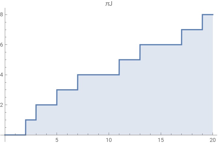
The Möbius inversion formula then gives: The sum is finite because for <2.
π(x)=J()=J()
∞
∑
n=1
μ(n)
n
1/n
x
log(2,x)
∑
n=1
μ(n)
n
1/n
x
J()=0
1/n
x
1/n
x
In[]:=
πJ[x_]:=SumMoebiusMu[n]Jπ[]n,{n,1,Log[2,x]}
1/n
x
Example:
In[]:=
πJ[100]
Out[]=
25
In[]:=
Plot[πJ[x],{x,0,20},Filling->Axis,PlotLabel->"πJ"]
Out[]=
Riemann gave an explicit formula for : for
J(x)
J(x)=Li(x)-Li()+t-log(2)
∑
ρ
ρ
x
∞
∫
x
1
t(-1)logt
2
t
x>1
Li(x)
Out[]=
Ei(x)
Out[]=
This is an usefull identity:
Out[]=
The main result of this notebook is the following identity:(*) t=-Ei(-2nlogx) for
∞
∫
x
1
t(-1)logt
2
t
∞
∑
n=1
x>1
First we calculate a series expansion around ∞ of the integrand:
In[]:=
Series,{t,∞,10}
1
t(-1)Log[t]
2
t
Out[]=
1
Log[t]
3
t
1
Log[t]
5
t
1
Log[t]
7
t
1
Log[t]
9
t
11
O
1
t
Now we integrate termwise:
In[]:=
Integrate,{t,x,∞},Assumptions->x>1
1
Log[t]
3
t
Out[]=
-ExpIntegralEi[-2Log[x]]
In[]:=
Integrate,{t,x,∞},Assumptions->x>1
1
Log[t]
5
t
Out[]=
-ExpIntegralEi[-4Log[x]]
So we conclude ():
x>1
Out[]=
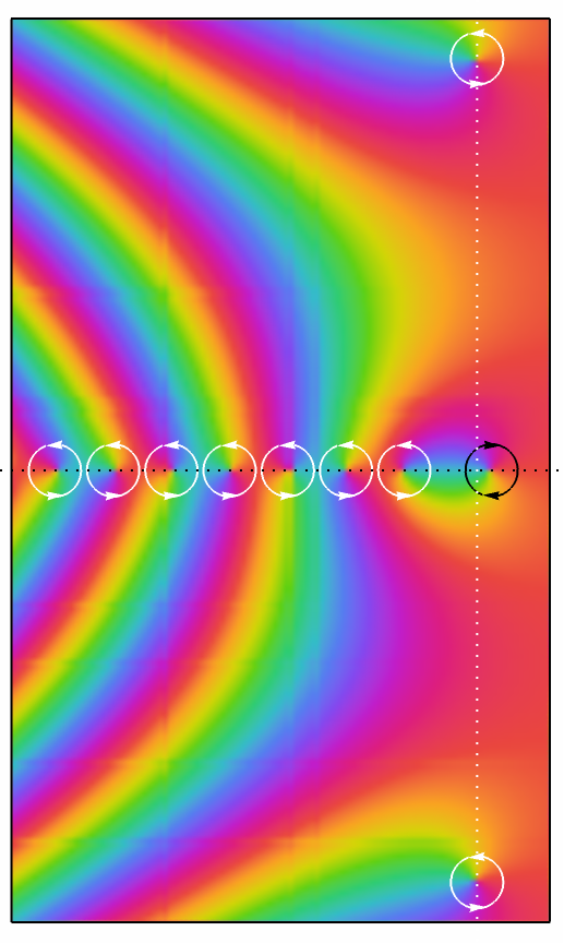
Now you can see, that , are the trivial zeros of the Zeta function:
-2n
nϵ
In[]:=
{Zeta[-2],Zeta[-4]}
Out[]=
{0,0}
The non trivial zeros are called with :
ρ
Imρ≠0
In[]:=
{N[ZetaZero[1]],Zeta[ZetaZero[1]]}
Out[]=
{0.5+14.1347,0}
Here you can see some zeros and the simple pole in the complex plane:
Out[]=
Some zeros and the pole of the Zeta function |
The first term is caused by the simple pole of Zeta at 1:
The second term is caused by the non trivial zeros and the third term is caused by the trivial zeros of the Zeta function. The forth term is simply:
or if you prefer the RiemannXi function:
Here is a working example:
Here 20 nontrivial zeros and 2 trivial zeros are used:
Here the Möbius inversion formula is again used:
Here 10 nontrivial zeros and 1 trivial zero are used:
Appendix PrimePi table:
Appendix PrimePi table:
CITE THIS NOTEBOOK
CITE THIS NOTEBOOK
Riemann's explicit formula made more explicit
by Oliver Seipel
Wolfram Community, STAFF PICKS, January 3, 2024
https://community.wolfram.com/groups/-/m/t/3095772
by Oliver Seipel
Wolfram Community, STAFF PICKS, January 3, 2024
https://community.wolfram.com/groups/-/m/t/3095772