For high quality video and discussion see:
𝓜𝐚𝐧𝐝𝐞𝐥𝐛𝐫𝐨𝐭 fractal encodes 𝓙𝐮𝐥𝐢𝐚 fractals.
Key animation developed: 𝐰𝐡𝐢𝐭𝐞 𝐝𝐨𝐭 in 𝓜 defines connectivity of 𝓙.
Despite few-symbol definition 𝐙 ↦ 𝐙²+𝐂 no finite computation exhausts an infinite fractal. Any algorithm gives only approximations. When facing infinitely intricate, infinitely explorable universes, the power of mathematical abstraction is to encode infinite in finite symbolic form. A few fun facts:
Both 𝓜𝐚𝐧𝐝𝐞𝐥𝐛𝐫𝐨𝐭 and 𝓙𝐮𝐥𝐢𝐚 fractals are defined as 𝐙 ↦ 𝐙²+ 𝐂
The difference? 𝓜 plots 𝐂, and 𝓙 plots 𝐙.
The white dot (parameter 𝐂) travels in 𝓜 set (corners) and the corresponding 𝓙 set is plotted in the center.
The difference? 𝓜 plots 𝐂, and 𝓙 plots 𝐙.
The white dot (parameter 𝐂) travels in 𝓜 set (corners) and the corresponding 𝓙 set is plotted in the center.
Thus: 𝓜𝐚𝐧𝐝𝐞𝐥𝐛𝐫𝐨𝐭 is an atlas for 𝓙𝐮𝐥𝐢𝐚.
It means each point 𝐂 (white dot) in 𝓜 set tells you the structure of the corresponding 𝓙 set. If white dot inside 𝓜 then 𝓙(𝐂) is one connected whole. If white dot outside 𝓜 then 𝓙(𝐂) shatters into dust. So the Mandelbrot works like a map: by scanning parameter space 𝐂, you can classify every possible Julia set for connectivity.
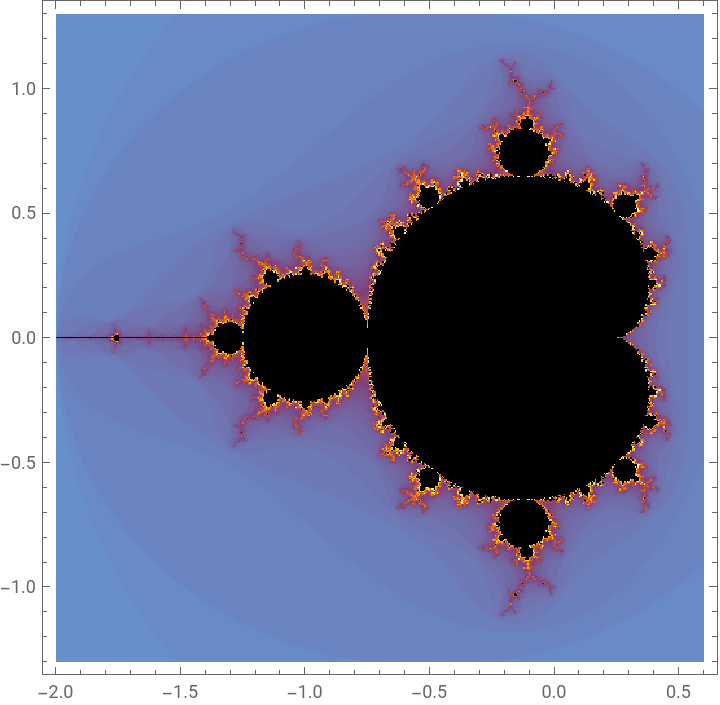
In Wolfram Language simplest code can plot these fractals. For example, functions below helped to make this video. Plot Mandelbrot:
In[]:=
MandelbrotSetPlot[]
Out[]=
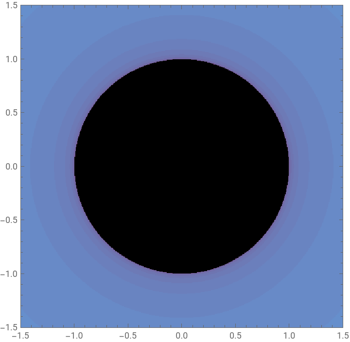
or even create interactive apps for Julia:
In[]:=
Manipulate[JuliaSetPlot[Complex@@p,PlotRange->1.5],{p,Locator},SaveDefinitions->True]
Out[]=

Assign a value of 550 for the image size parameter in subsequent plots or visualizations:
In[]:=
grSZ=550;
A list of 13 two-dimensional points is defined. These give nice Julia images.
In[]:=
pts={{-0.205,0.686},{-0.297,0.648},{-0.216,0.707},{-0.2,0.806},{-0.117,0.862},{-0.203,0.811},{-0.218,0.712},{-0.285,0.638},{-0.186,0.653},{-0.086,0.658},{-0.087,0.668},{-0.187,0.673},{-0.187,0.663}};
A B-spline function is created using this set of points. This function represents a smooth curve that interpolates the given points. It is defined to be closed, meaning the start and end points of the curve are connected.
In[]:=
bsp=BSplineFunction@@ResourceFunction["CubicSplineCurve"][pts,SplineClosed->True]
Out[]=
BSplineFunction


A function is defined to plot the Mandelbrot set, which is a fractal that is used in complex dynamics. The plot includes a small white disk at a specified position, possibly for highlighting a point of interest. THis will serve as inset later.
In[]:=
mand[p_]:=MandelbrotSetPlot[ColorFunction->"SunsetColors",Frame->False,ImageSize->grSZ/3.,Epilog->{White,Disk[p,.01]},PlotRange->{{-.4,0},{.6,1}},PerformanceGoal->"Quality"]mand[{-.35,.7}]
Out[]=

In[]:=
mand2[p_]:=MandelbrotSetPlot[ColorFunction->"SunsetColors",Frame->False,ImageSize->grSZ/3.,Epilog->{White,Disk[p,.05]},PerformanceGoal->"Quality"]mand2[{-.35,.7}]
Out[]=
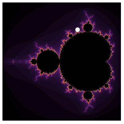
A function is used to create an interactive plot of the Julia set, which is another type of fractal related to complex numbers. It includes insets of the Mandelbrot set plots created earlier, with the highlighted points dynamically calculated based on the B-spline function. The visualization allows the user to explore different Julia sets by adjusting a parameter.
In[]:=
Manipulate[JuliaSetPlot[Complex@@bsp[t],ImageSize->grSZ{1,1},PerformanceGoal->"Quality",PlotRange->1.4,Frame->False,Epilog->{Inset[mand[bsp[t]],{Right,Top},{Right,Top}],Inset[mand2[bsp[t]],{Left,Bottom},{Left,Bottom}]}],{t,0,1},SaveDefinitions->True]
Out[]=


CITE THIS NOTEBOOK
CITE THIS NOTEBOOK
Two views of z ↦ z² + c: Mandelbrot set fractal charts connectivity of related Julia set fractal
by Vitaliy Kaurov
Wolfram Community, STAFF PICKS, September 11, 2025
https://community.wolfram.com/groups/-/m/t/3543860
by Vitaliy Kaurov
Wolfram Community, STAFF PICKS, September 11, 2025
https://community.wolfram.com/groups/-/m/t/3543860