ABSTRACT (original article): The presence of topological flat minibands in moiré materials provides an opportunity to explore the interplay between topology and correlation. In this work, we study moiré minibands in topological insulator films with two hybridized surface states under a moiré superlattice potential created by two-dimensional insulating materials. We show the lowest conduction (highest valence) Kramers’ pair of minibands can be non-trivial when the minima (maxima) of moiré potential approximately form a hexagonal lattice with six-fold rotation symmetry. Coulomb interaction can drive the non-trivial Kramers’ minibands into the quantum anomalous Hall state when they are half-filled, which is further stabilized by applying external gate voltages to break inversion. We propose the monolayer Sb2 on top of Sb2Te3 films as a candidate based on first principles calculations. Our work demonstrates the topological insulator based moiré heterostructure as a potential platform for studying interacting topological phases. CITATION (original article): Yang, K., Xu, Z., Feng, Y. et al. Topological minibands and interaction driven quantum anomalous Hall state in topological insulator based moiré heterostructures. Nature Communications 15, 2670 (2024). https://doi.org/10.1038/s41467-024-46717-7
Introduction
Introduction
This notebook presents a theoretical study of the electronic properties of moiré materials based on topological insulators. We introduce the continuum model Hamiltonian for a topological insulator thin film under a moiré superlattice potential and study the surface electronic bands of the topological insulator under moiré Brillouin zone folding. We focus on the topological aspects of the electronic bands and calculate the nontrivial topological invariants by the Wannier center flow. Besides, due to the small bandwidth compared with the Coulomb interaction between electrons, several strong correlation phases are identified based on Hartree Fock mean field methods. Our notebook serves as a numerical toolbox for researchers interested in the moiré systems, topology, and strong correlation physics.
2
Continuum Hamiltonian
Continuum Hamiltonian
This section constructs the continuum model Hamiltonian in the momentum space for the surface states of a topological insulator thin film under the moiré potential as formulated in Equation (1) of the main text.
We begin by the Hamiltonian of the surface states in Equation (1) in the atomic lattice without moiré potential.
TI
H
In[]:=
hamti[{kx_,ky_},{v_,m_}]:={{0,v(kx-ky),Conjugate@m,0},{-v(kx+ky),0,0,Conjugate@m},{m,0,0,-v(kx-ky)},{0,m,v(kx+ky),0}}
We define the moiré Brillouin zone in the momentum space.
In[]:=
twistangle=0.5π/180;scaling=0;
In[]:=
b1moire=scaling-,+twistangle,;b2moire=scaling-,-+twistangle-,;kG={0,0};kK=(b1moire+b2moire)/3;kM=b1moire/2;
4π
3
3
2
1
2
4π
3
1
2
3
2
4π
3
3
2
1
2
4π
3
1
2
3
2
We define the moiré potential in the momentum space.
Δ(r)
In[]:=
vg0=2.654/4.36;tinterlayerg0=0.0498;tinterlayerg1=-0.00437+0.00805;
In[]:=
ClearAll[moirepotential];
In[]:=
nflatband=2*Length@glist;energyscale=(vg0Norm@b1moire);
In[]:=
(*moirepotential*)moirepotential[{tg0_,tg1_,alpha_}]:=moirepotential[{tg0,tg1,alpha}]=ArrayFlatten@Outer[Switch[#2-#1,(*〈k|H|k〉*){0,0},tg0KroneckerProduct[DiagonalMatrix[{1,(*alpha*)-1}],IdentityMatrix[2]],(*〈k|H|k+g1〉*){1,0},tg1KroneckerProduct[DiagonalMatrix[{1,alpha}],IdentityMatrix[2]],(*〈k|H|k+g2〉*){0,1},ConjugateTranspose[tg1KroneckerProduct[DiagonalMatrix[{1,alpha}],IdentityMatrix[2]]],(*〈k|H|k-g1〉*){-1,0},ConjugateTranspose[tg1KroneckerProduct[DiagonalMatrix[{1,alpha}],IdentityMatrix[2]]],(*〈k|H|k-g2〉*){0,-1},tg1KroneckerProduct[DiagonalMatrix[{1,alpha}],IdentityMatrix[2]],(*〈k|H|k+g1-g2〉*){1,-1},ConjugateTranspose[tg1KroneckerProduct[DiagonalMatrix[{1,alpha}],IdentityMatrix[2]]],(*〈k|H|k-g1+g2〉*){-1,1},tg1KroneckerProduct[DiagonalMatrix[{1,alpha}],IdentityMatrix[2]],_,0IdentityMatrix[4]]&,glist,glist,1]
We add the and Δ(r) together and formulates the continuum model with a cutoff by glist.
TI
H
In[]:=
glist=Prepend[Join@@Table[Union@Flatten[Table[{n-i,i}.b,{b,Partition[{{0,1},{1,0},{1,-1},{0,-1},{-1,0},{-1,1}},2,1,1]},{i,0,n}],1],{n,1,5}],{0,0}];
In[]:=
blockArray[mat_]:=SparseArray[Tuples[Range@#-{1,0,0}].{Rest@#,{1,0},{0,1}}&@Dimensions@matFlatten@mat]
In[]:=
hammoire[k_List,pti_,pinter_]:=blockArray[Table[hamti[k+g.{b1moire,b2moire},pti],{g,glist}]]+moirepotential[pinter]
Electronic bands
Electronic bands
In this section, we plot the electronic band structure of the continuum model in the moiré Brillouin zone.
The in moiré Brillouin zone for plotting the band structure.
Γ-K-M
In[]:=
ks=With[{dk=N[Norm[kG-kK]/30,MachinePrecision]},Join[Table[kG+λ(kK-kG),{λ,0,1,dk/Norm[kG-kK]}],Rest@Table[kK+λ(kM-kK),{λ,0,1,dk/Norm[kM-kK]}]]];
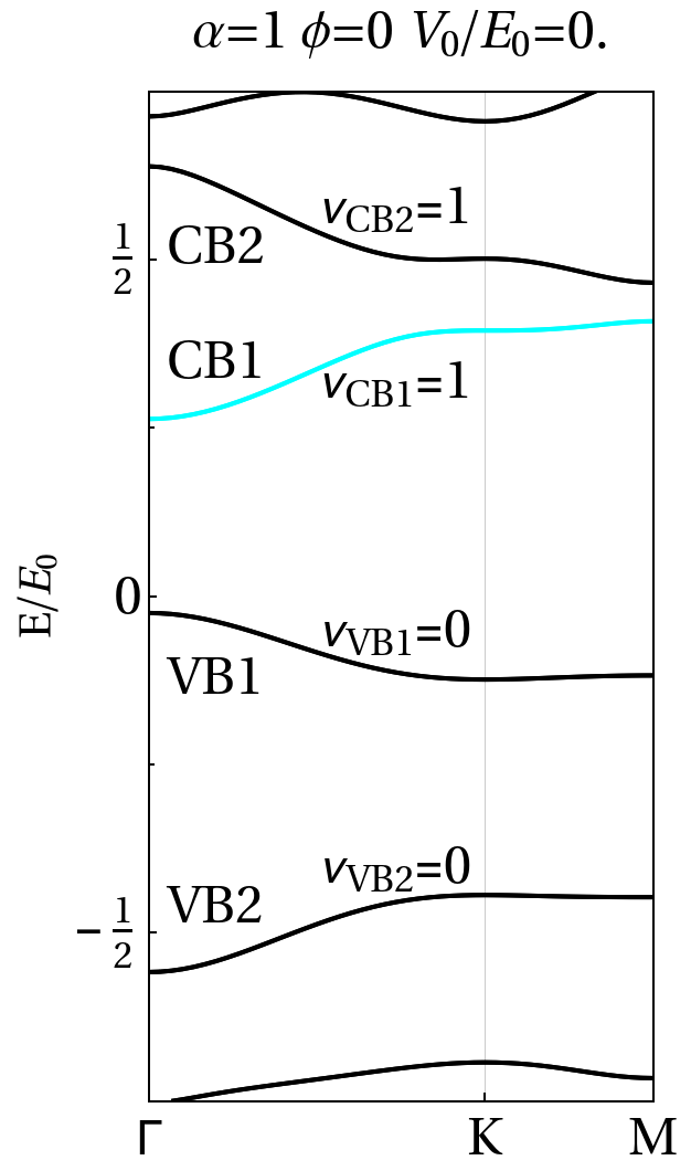
We plot the example band structures with the topologically nontrivial lowest conduction band CB1 in regime I of Figure 2c in the main text.
In[]:=
deltaphi=0;parametermoire={0energyscale,1Abs[tinterlayerg1]Exp[2πdeltaphi],1};parameterti={vg0,0.4energyscale};
In[]:=
xtickspectrum=Transpose@{With[{dk=N[Norm[kG-kK]/30,MachinePrecision]},Length/@{{0},Join[Range[0,1,dk/Norm[kK-kG]]],ks}],{"Γ","K","M"}};ytickspectrum=Table[{x,x,{0.015,0}},{x,Chop@Subdivide[-1,4,10]}]~Join~Table[{x," ",{0.01,0}},{x,Chop@Subdivide[-1,4,20]}];ytick2spectrum=Table[{x," ",{0.015,0}},{x,Chop@Subdivide[-1,4,10]}]~Join~Table[{x," ",{0.01,0}},{x,Chop@Subdivide[-1,4,20]}];spectrum=Part[Transpose@Table[Sort@Eigenvalues@hammoire[k,parameterti,parametermoire],{k,ks}]/energyscale,nflatband-15;;nflatband+32];
In[]:=
styletext=Directive[Black,FontFamily"Times New Roman",FontSizeLarge];
In[]:=
styleframe=Sequence[FrameTrue,LabelStylestyletext,FrameTicksStylestyletext,FrameStyleDirective[Black,Thickness[Medium]],ImageSizeMedium];
In[]:=
Show[ListLinePlot[spectrum,PlotRange{{1,Length@ks},{-3/4,3/4}},GridLines{First/@xtickspectrum,None},AspectRatio->2,Axes->False,PlotLabel"α="<>ToString[Last@parametermoire]<>" ϕ="<>ToString[deltaphi,FormatTypeStandardForm]<>" /="<>ToString[N[parametermoire[[1]]/energyscale,2]],PlotStyleJoin[ConstantArray[Black,4],ConstantArray[Cyan,2],ConstantArray[Black,6]],PlotRangePaddingNone,FrameTicks{{ytickspectrum,None},{xtickspectrum,None}},FrameLabel{{"E/",None},{None,None}},LabelStyleDirective[Black,FontSize20,FontFamily"Times"],styleframe],Graphics[{Text["=1"~Style~styletext,{23,0.32}],Text["=1"~Style~styletext,{23,0.58}],Text["=0"~Style~styletext,{23,-0.05}],Text["=0"~Style~styletext,{23,-0.4}],Text["CB1"~Style~styletext,{7,0.35}],Text["CB2"~Style~styletext,{7,0.52}],Text["VB1"~Style~styletext,{7,-0.12}],Text["VB2"~Style~styletext,{7,-0.46}]}],ImageSizeMedium]
V
0
E
0
E
0
ν
CB1
ν
CB2
ν
VB1
ν
VB2
Out[]=
We plot the example band structures with topologically nontrivial CB1 in regime II of Figure 2c in the main text.
In[]:=
deltaphi=0;parametermoire={1.2energyscale,1Abs[tinterlayerg1]Exp[2πdeltaphi],0};parameterti={vg0,0.4energyscale};
In[]:=
xtickspectrum=Transpose@{With[{dk=N[Norm[kG-kK]/30,MachinePrecision]},Length/@{{0},Join[Range[0,1,dk/Norm[kK-kG]]],ks}],{"Γ","K","M"}};ytickspectrum=Table[{x,x,{0.015,0}},{x,Chop@Subdivide[-1,4,10]}]~Join~Table[{x," ",{0.01,0}},{x,Chop@Subdivide[-1,4,20]}];ytick2spectrum=Table[{x," ",{0.015,0}},{x,Chop@Subdivide[-1,4,10]}]~Join~Table[{x," ",{0.01,0}},{x,Chop@Subdivide[-1,4,20]}];spectrum=Part[Transpose@Table[Sort@Eigenvalues@hammoire[k,parameterti,parametermoire],{k,ks}]/energyscale,nflatband-15;;nflatband+32];
In[]:=
Show[ListLinePlot[spectrum,PlotRange{{1,Length@ks},{-1/2,1/2}},GridLines{First/@xtickspectrum,None},AspectRatio->2,Axes->False,PlotLabel"α="<>ToString[Last@parametermoire]<>" ϕ="<>ToString[deltaphi,FormatTypeStandardForm]<>" /="<>ToString[N[parametermoire[[1]]/energyscale,2]],PlotStyleJoin[ConstantArray[Black,4],ConstantArray[Cyan,2],ConstantArray[Black,6]],PlotRangePaddingNone,FrameTicks{{ytickspectrum,None},{xtickspectrum,None}},FrameLabel{{"E/",None},{None,None}},LabelStyleDirective[Black,FontSize20,FontFamily"Times"],styleframe],Graphics[{Text["=1"~Style~styletext,{23,0.28}],Text["=0"~Style~styletext,{23,0.46}],Text["=0"~Style~styletext,{23,-0.07}],Text["=0"~Style~styletext,{23,-0.15}],Text["CB1"~Style~styletext,{7,0.30}],Text["CB2"~Style~styletext,{7,0.42}],Text["VB1"~Style~styletext,{7,-0.12}],Text["VB2"~Style~styletext,{7,-0.25}]}],ImageSizeMedium]
V
0
E
0
E
0
ν
CB1
ν
CB2
ν
VB1
ν
VB2
Wannier center flow
Wannier center flow
We first define the Wilson loop function.
Hartree Fock Mean Field Two Band
Hartree Fock Mean Field Two Band
In this section, we use the Hartree Fock mean field method to study the interacting phases at the half filling of CB1.
We first define a momentum mesh in Brillouin zone for calculation of various integrals over Brillouin zone.
We define the dual gated screened Coulomb potential in Equation (52) of the supplementary note.
Then, we project the Coulomb interaction and non interacting Hamiltonian into the two band basis of CB1 as formulated in supplementary note 2 section A.
We use the density matrix as the order parameters for the Hartree Fock mean field method and prepare two types of initial density matrix as formulated in supplementary note 2 section C, (i) the mirror polarized phase and (ii) the mirror coherent density matrix.
The self-consistent Hartree Fock formulated in supplementary note 2 section B is implemented. The code is run over multiple times until the convergence of Hartree Fock mean field spectrum.
Finally, the condensation energy is calculated for two types of interacting phases and the mirror polarized phase, which has the lowest condensation energy, is the ground state.
Hartree Fock Mean Field Two Band Data on a dense BZ mesh
Hartree Fock Mean Field Two Band Data on a dense BZ mesh
In this section, we present the Hartree Fock mean field results in the parameter Regime I and II of Figure 2c in the main text.
We first plot the Hartree Fock mean field spectrum of the mirror polarized phase with parameters in Regime I.
The mirror polarized phase has a gap opened between two bands of CB1 and the filled lower energy band has nonzero Chern number.
The mirror polarized phase has a gap opened between two bands of CB1 and the filled lower energy band has nonzero Chern number.
We then plot the mean field spectrum of the mirror coherent phase with parameters in Regime I.
The mirror coherent phase has a node between two bands of CB1.
The mirror coherent phase has a node between two bands of CB1.
Finally, we compare the energy for two phases under different Coulomb interaction strength.
Upon a critical Coulomb interaction strength, a mirror polarized order parameter with nonzero Chern number starts to develop and becomes the ground state of the system.
Upon a critical Coulomb interaction strength, a mirror polarized order parameter with nonzero Chern number starts to develop and becomes the ground state of the system.
A similar analysis of the Hartree Fock mean field for two phases is done for the Hamiltonian parameter in Regime II.
The ground state of interacting CB1 still has nonzero Chern number.
The ground state of interacting CB1 still has nonzero Chern number.
Hartree Fock Mean Field Four Band Data on a dense BZ mesh
Hartree Fock Mean Field Four Band Data on a dense BZ mesh
In this section, we consider the band mixing effects into the Hartree Fock mean field by including higher energy conduction band CB2 to check the stability of the ground state with nonzero Chern number.
In Hamiltonian parameter regime I, we present the Hartree Fock mean field spectrum for the interaction strength in regime B and C of Figure 4a of the main text.
The Chern number of the ground state undergoes a topological phase transition by mixing CB2 when the coulomb interaction strength in regime C is larger than the gap between CB1 and CB2.
The Chern number of the ground state undergoes a topological phase transition by mixing CB2 when the coulomb interaction strength in regime C is larger than the gap between CB1 and CB2.
In Hamiltonian parameter regime II, we present the Hartree Fock mean field spectrum and the Chern number for the ground state is always nonzero.
The nonzero electrical field in Hamiltonian parameter regime II stabilizes the ground state with nonzero Chern number.
The nonzero electrical field in Hamiltonian parameter regime II stabilizes the ground state with nonzero Chern number.
Conclusion
Conclusion
CITE THIS NOTEBOOK
CITE THIS NOTEBOOK
Topological minibands and interaction driven quantum anomalous Hall state in topological insulator based moiré heterostructures
by Kaijie Yang, Zian Xu, Yanjie Feng, Frank Schindler, Yuanfeng Xu, Zhen Bi, B. Andrei Bernevig, Peizhe Tang & Chao-Xing Liu
Wolfram Community, STAFF PICKS, September 27, 2024
https://community.wolfram.com/groups/-/m/t/3288963
by Kaijie Yang, Zian Xu, Yanjie Feng, Frank Schindler, Yuanfeng Xu, Zhen Bi, B. Andrei Bernevig, Peizhe Tang & Chao-Xing Liu
Wolfram Community, STAFF PICKS, September 27, 2024
https://community.wolfram.com/groups/-/m/t/3288963
The article https://doi.org/10.1038/s41467-024-46717-7 is licensed under a Creative Commons Attribution 4.0 International License http://creativecommons.org/licenses/by/4.0/