This Wolfram notebook presents a kinematic analysis and animation of a quick return mechanism. It demonstrates the mechanism at two angular velocities (5 and 9 rad/s) with constant angular acceleration. A common application of quick return mechanisms is found in metal shapers .
Kinematic Parameters of a Quick Return Mechanism
Kinematic Parameters of a Quick Return Mechanism
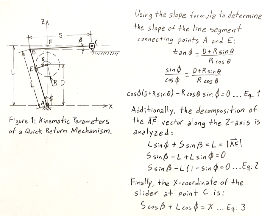
Position Equations
Position Equations
Clear[L,S,Dd,R,ϕ,θ,β,t];(*AssymbolDisprotected,thesymbolDdwillbeusedinstead*)Eq1=Cos[ϕ[t]](Dd+RSin[θ[t]])-RCos[θ[t]]Sin[ϕ[t]]==0;(*SeeFigure1*)Eq2=SSin[β[t]]-L(1-Sin[ϕ[t]])==0;(*SeeFigure1*)Eq3=SCos[β[t]]+LCos[ϕ[t]];(*SeeFigure1*)
Velocity Equations (ω = 9 rad/s)
Velocity Equations (ω = 9 rad/s)
Velocity Equations : Input angle (θ) is set as a known input value (9 t), and the angular velocity is set to 9 rad/s .
vE=Dt[{Eq1,Eq2},t,Constants{Dd,R,S,L}]/.{θ[t]->9t,[t]->9};
′
θ
Parameter Values for the mechanism
Parameter Values for the mechanism
Parameters from reference [1] : Fung, R . F ., & Chen, K . W . (1997) . Constant speed control of the quick return mechanism driven by a DC motor . JSME International Journal Series C Mechanical Systems, Machine Elements and Manufacturing, 40 (3), 454 - 461.
L=0.2222;S=0.2408;Dd=0.1294;R=0.0556;Hyperlink["Constant speed control of the quick return mechanism driven by a DC motor","https://www.jstage.jst.go.jp/article/jsmec1997/40/3/40_3_454/_pdf"]
Velocity Equations: Solutions and Plots (ω = 9 rad/s)
Velocity Equations: Solutions and Plots (ω = 9 rad/s)
From inspection of Figure 1, note that :
- When θ = 0, then ϕ = ArcTan[Dd/R] .
- When θ = π/2, then β = 0
- When θ = 0, then ϕ = ArcTan[Dd/R] .
- When θ = π/2, then β = 0
s1=NDSolvevE[[1]],vE[[2]],ϕ[0]==ArcTan[Dd/R],β==0,{ϕ,β},{t,0,6π}
π
2
Out[]=
ϕInterpolatingFunction,βInterpolatingFunction


In[]:=
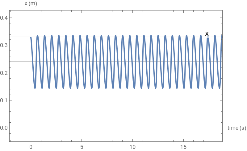
Plot[Evaluate[Eq3/.s1],{t,0,6π},PlotLabelsPlaced[{"X"},Above],FrameTrue,AxesLabel{"time (s)","x (m)"},Axes->True,AxesOrigin{0,0},PlotRange{{-2.1,6π},{-.05,.4}},GridLines->{{3π/2},{S,0.145,0.3325}},ImageSize->400](*Plotofsliderstroke.Sliderlimitsaresetto0.145and0.3325accordingtoreference[1]*)
Out[]=
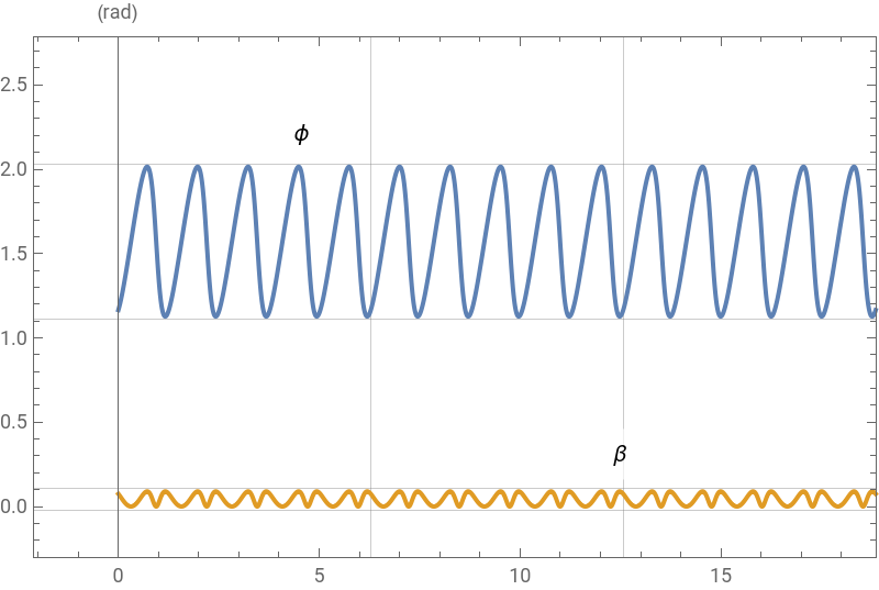
Plot of Angles ϕ and β
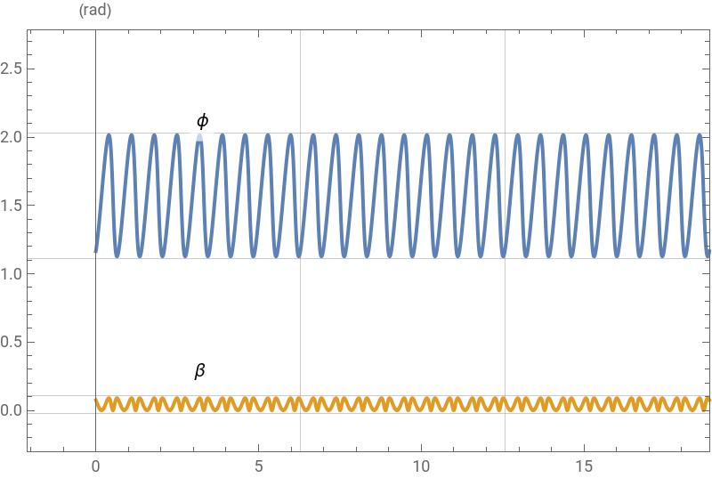
Plot[Evaluate[{ϕ[t],β[t]}/.s1],{t,0,6π},PlotLabelsPlaced[{"ϕ","β"},Above],FrameTrue,AxesLabel{"time (s)","(rad)"},Axes->True,AxesOrigin{0,0},PlotRange{{-2.1,6π},{-.3,2.5}},GridLines->{{2π,4π},{-.02,0.11,1.11,2.03}},ImageSize->400]
Out[]=
Velocity Equations (ω = 5 rad/s)
Velocity Equations (ω = 5 rad/s)
Velocity Equations : Input angle (θ) is set as a known input value (5 t), and the angular velocity is set to 5 rad/s.
vE2=Dt[{Eq1,Eq2},t,Constants{Dd,R,S,L}]/.{θ[t]->5t,[t]->5};
′
θ
Velocity Equations: Solutions and Plots (ω = 5 rad/s)
Velocity Equations: Solutions and Plots (ω = 5 rad/s)
Again, from inspection of Figure 1, note that :
- When θ = 0, then ϕ = ArcTan[Dd/R] .
- When θ = π/2, then β = 0
- When θ = 0, then ϕ = ArcTan[Dd/R] .
- When θ = π/2, then β = 0
s2=NDSolve[{vE2[[1]],vE2[[2]],ϕ[0]==ArcTan[Dd/R],β[π/2]==0},{ϕ,β},{t,0,6π}];
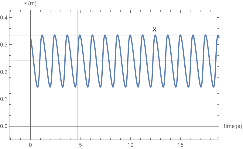
Plot of slider stroke . Slider limits are set to 0.145 and 0.3325 according to reference[1]
Plot[Evaluate[Eq3/.s2],{t,0,6π},PlotLabelsPlaced[{"X"},Above],FrameTrue,AxesLabel{"time (s)","x (m)"},Axes->True,AxesOrigin{0,0},PlotRange{{-2.1,6π},{-.05,.4}},GridLines->{{3π/2},{S,0.145,0.3325}},ImageSize->400]
Out[]=
Plot of Angles ϕ and β
Plot[Evaluate[{ϕ[t],β[t]}/.s2],{t,0,6π},PlotLabelsPlaced[{"ϕ","β"},Above],FrameTrue,AxesLabel{"time (s)","(rad)"},Axes->True,AxesOrigin{0,0},PlotRange{{-2.1,6π},{-.3,2.5}},GridLines->{{2π,4π},{-.02,0.11,1.11,2.03}},ImageSize->400]
Out[]=
Animation
Animation
References
References
CITE THIS NOTEBOOK
CITE THIS NOTEBOOK
Kinematic analysis and animation of a quick return mechanism
by David Balandra
Wolfram Community, STAFF PICKS, February 27, 2024
https://community.wolfram.com/groups/-/m/t/3131236
by David Balandra
Wolfram Community, STAFF PICKS, February 27, 2024
https://community.wolfram.com/groups/-/m/t/3131236