CITE THIS NOTEBOOK: Modeling supply and demand in Economics by Sangdon Lee. Wolfram Community OCT 14 2022.
CITE THIS NOTEBOOK: Modeling supply and demand in Economics by Sangdon Lee. Wolfram Community OCT 14 2022.
Introduction
Introduction
This is an example on how to model the supply and demand in economics. I will use this model to simulate how long it will take if normal supply quantity is suddenly reduced from 100 units/month to 90 units/month (e.g., Plants were shutdown due to corona virus.)
Core structure of supply and demand:
Core structure of supply and demand:
The core structure of supply demand is the feedback loops among the supply, demand, inventory and price that create dynamics;
(1) inventory level affects price (i.e., plentiful of inventory will lower price) (2) the difference between supply and demand quantity changes price and in turn (3) the changed price will adjust the supply and demand quantity (i.e., people will be hesitant to purchase due to higher price).
(1) inventory level affects price (i.e., plentiful of inventory will lower price) (2) the difference between supply and demand quantity changes price and in turn (3) the changed price will adjust the supply and demand quantity (i.e., people will be hesitant to purchase due to higher price).
◼
It is critical to note that (1) inventory (e.g., cars) and (2) price (e.g., $/cars) are state variables and (1) Supply (e.g., cars/month) and(2) demand(e.g., cars/month) are flow variables. Their units of measurements are different.
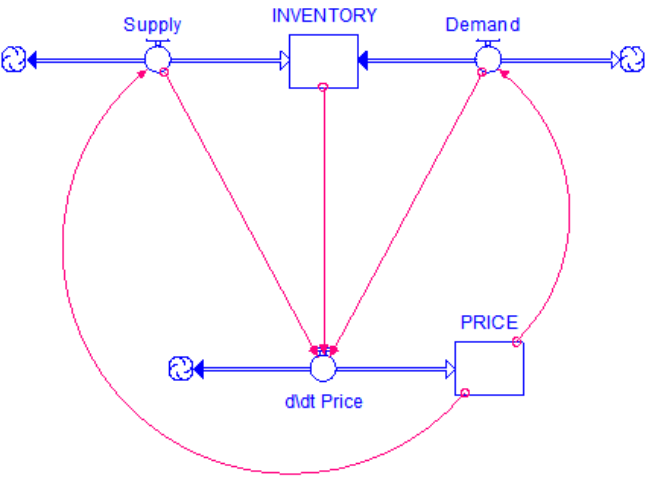
The core structure can be expressed in (1) System Dynamics equation form (or integration equation form) or (2) differential equation form, which are equivalent, but I found that SD form is easier to understand.
System Dynamics form or Integration equation form:
System Dynamics form or Integration equation form:
(* e.g., inventory at next month, t + dt, is equal to the inventory at this month, t, and increased by supply and decreased by demand in 1 month period *)
INVENTORY(t+dt)=INVENTORY(t)+(supply(t)-demand(t))*dt=INVENTORY(t)+(coefficient1*PRICE(t)-coefficient2*PRICE(t))*dtPRICE(t+dt)=PRICE(t)+(-coefficient3*INVENTORY(t)+coefficient4*(supply(t)-demand(t)))*dt=PRICE(t)+(-coefficient3*INVENTORY(t)+coefficient4*(coefficient1*PRICE(t)-coefficient2*PRICE(t)))*dt
Differential equation form:
Differential equation form:
INVENTORY(t)
t
PRICE(t)
t
Traditional graphical representation
Traditional graphical representation
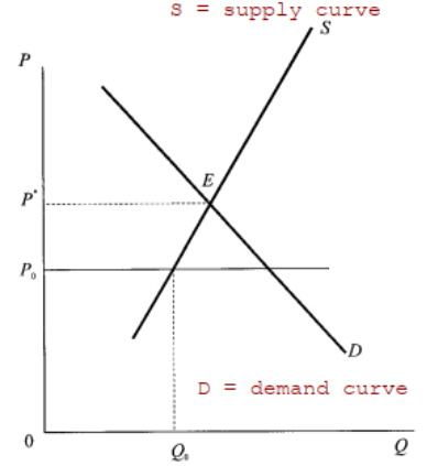
Supply and demand is usually explained using the following graph which does not explain well how the inventory (or quantity, Q), price, supply and demand will change over time.
Stock and Flow Diagram for Supply and demand :
Stock and Flow Diagram for Supply and demand :
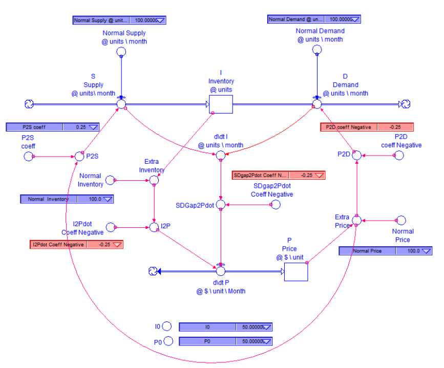
The core structure is expanded as shown below. I include normal quantities of inventory, price, supply and demand. This model assumes that the various effects of inventory and price are linear, that is, proportional to inventory and price. Stock, flow, and parameters have units of measurements after @: e.g. Inventory @ units.
Note that the various coefficients in dimensionless fractions (e.g.,c1 P2S = 0.25) can be better understood if they are converted into time to adjust. The time to adjust indicates the time duration it takes for the step response to rise up to 63% or 0.63 of its final value.
Note that the various coefficients in dimensionless fractions (e.g.,c1 P2S = 0.25) can be better understood if they are converted into time to adjust. The time to adjust indicates the time duration it takes for the step response to rise up to 63% or 0.63 of its final value.
Modeling using ParametricNDSolve
Modeling using ParametricNDSolve
In[]:=
sol=ParametricNDSolve[{tMax=100;(*statevariables*)INVENTORY'[t]==+supply[t]-demand[t],PRICE'[t]==-c3SDGap2P*sdGap[t]-c4I2P*extraInventory[t](*c3SDGap2P=coefficient3fromsupply-damandgaptoprice*)(*c4I2P=coefficient4frominventorytoprice*),(*auxiliaryvariables*)supply[t]==c1P2S*extraPrice[t]+normalSupply[t](*c1P2S=coefficient1frompricetosupply*),demand[t]==c2P2D*extraPrice[t]+normalDemand(*c2P2S=coefficient2frompricetodemand*),extraPrice[t]==PRICE[t]-normalPrice,extraInventory[t]==INVENTORY[t]-normalInventory,sdGap[t]==supply[t]-demand[t](*differencebetweensuppplyanddemandquantity*),normalSupply[t]==100-UnitStep[t-10]*10(*normalsupplyisreducedfrom100to90units/month*),(*initialvalues.Notethatauxiliaryvariableshavenoinitialvalues*)INVENTORY[0]==i0,PRICE[0]==p0},(*stateandauxiliaryvariabels*){INVENTORY,PRICE,supply,demand,extraPrice,extraInventory,sdGap,normalSupply},{t,0,tMax}(*simulationperiod.NotethatthetMaxislongerthanthePlotRange*),(*parameterstochange*){c1P2S,c2P2D,c3SDGap2P,c4I2P,normalDemand,normalPrice,normalInventory,i0,p0}];
Simulation
Simulation
In[]:=
Manipulate[{(*1supply&demandovertime*)Plot[Evaluate[{normalSupply[c1P2S,c2P2D,c3SDGap2P,c4I2P,normalDemand,normalPrice,normalInventory,i0,p0][t]/.sol,normalDemand}],{t,0,50},Frame->True,FrameLabel->"Month",PlotLegends->Placed[{"Normal Supply (cars/month)","Normal Demand (cars/month)"},Above],PlotRange->{All,{80,120}},ImageSize->250,GridLines->Automatic],(*2inventory&priceovertime*)Plot[Evaluate[{INVENTORY[c1P2S,c2P2D,c3SDGap2P,c4I2P,normalDemand,normalPrice,normalInventory,i0,p0][t]/.sol,PRICE[c1P2S,c2P2D,c3SDGap2P,c4I2P,normalDemand,normalPrice,normalInventory,i0,p0][t]/.sol}],{t,0,50},FrameTrue,FrameLabel"Month",PlotLegendsPlaced[{"INVENTORY (cars)","PRICE($/car)"},Above],PlotRange{All,{50,150}},ImageSize250,GridLines->Automatic],(*3inventoryvsprice*)ParametricPlot[Evaluate[{PRICE[c1P2S,c2P2D,c3SDGap2P,c4I2P,normalDemand,normalPrice,normalInventory,i0,p0][t]/.sol,INVENTORY[c1P2S,c2P2D,c3SDGap2P,c4I2P,normalDemand,normalPrice,normalInventory,i0,p0][t]/.sol}],{t,0,50},Frame->True,FrameLabel->{"PRICE ($/car)","INVENTORY (cars/month)"},PlotRange->{{50,150},{50,150}},ImageSize->200,AspectRatio->1,GridLines->Automatic],(*4supplyanddemandGap*)Plot[Evaluate[{supply[c1P2S,c2P2D,c3SDGap2P,c4I2P,normalDemand,normalPrice,normalInventory,i0,p0][t],demand[c1P2S,c2P2D,c3SDGap2P,c4I2P,normalDemand,normalPrice,normalInventory,i0,p0][t]}/.sol],{t,0,50},Frame->True,FrameLabel->"Month",PlotLegends->Placed[{"Supply (cars/month)","Demand (cars/month)"},Above],PlotRange->{All,{80,120}},ImageSize->250,GridLines->Automatic],(*5pricevsdemand*)ParametricPlot[Evaluate[{PRICE[c1P2S,c2P2D,c3SDGap2P,c4I2P,normalDemand,normalPrice,normalInventory,i0,p0][t],demand[c1P2S,c2P2D,c3SDGap2P,c4I2P,normalDemand,normalPrice,normalInventory,i0,p0][t]}/.sol],{t,0,50},Frame->True,FrameLabel->{"PRICE ($/cars)","Demand(cars/month)"},PlotRange->{All,{80,120}},ImageSize->200,AspectRatio->1,GridLines->Automatic],(*6.pricevssupply*)ParametricPlot[Evaluate[{PRICE[c1P2S,c2P2D,c3SDGap2P,c4I2P,normalDemand,normalPrice,normalInventory,i0,p0][t],supply[c1P2S,c2P2D,c3SDGap2P,c4I2P,normalDemand,normalPrice,normalInventory,i0,p0][t]}/.sol],{t,0,50},Frame->True,FrameLabel->{"PRICE ($/cars)","Supply(cars/month)"},PlotRange->{{50,150},{50,150}},ImageSize->200,AspectRatio->1,GridLines->Automatic]},"Normal supply is decreased from 100 to 90 cars/month at t = 10 month",Delimiter,{{c4I2P,0.25,"Coeff:\nInventory -> Price"},0.0,1.0,0.05},{{c3SDGap2P,0.25,"Coeff: \nSupply & Demand Gap -> Price"},0.0,1.0,0.05},Delimiter,{{c1P2S,0.25,"Coeff:\nPrice -> Supply"},0.0,1.0,0.05},{{c2P2D,-0.25,"Coeff:\nPrice -> Demand"},-1.0,0.0,0.05},Delimiter,{{normalInventory,100,"Normal Inventory Level\n(cars/m)"},0,200,5},{{normalDemand,100,"Normal Demand Level \n(cars/m)"},0,200,5},{{normalPrice,100,"($/m)"},0,200,5},Delimiter,{{i0,100},0,200,5},{{p0,100},0,200,5},ControlPlacementLeft,SaveDefinitions->True]
Summary
Summary
◼
The normal supply is decreased from 100 cars/month to 90 cars/month, and the normal demand remains unchanged. As the inventory level drops, the price increases which will then increase the supply quantity and reduce the demand with time delay. Eventually the inventory level returns to normal inventory level and the price is increased from 100 to 120 $/car
◼
The difference between supply and demand quantity has an effect of dampening the price (i.e., d/dt Inventory[t] ). This is similar to the damping force in mass-spring-damper system
◼
(1) Price to supply, (2) price to demand, and (3) inventory to price make the price and inventory fluctuate. They are similar to the spring force in mass-spring-damper system
◼
Coefficients indicate time delay! Note that the coefficients for these effects are fractions or percentage. For example, “Coeff: Inventory -> Price” is set at 0.25, which is equivalent to 1/time to adjust =0.25 -> 4 days, thus it will take 4 days for the actual inventory to reach 63% of step input of 100. In other words, coefficient indicates” time delay!. Time delay is one of the most disturbing factor creating fluctuation as well as feedback loops.
◼
Improvements
◼
Make coefficients to be endogenous or nonlinear (e.g., non-linear spring or damping coefficients),
◼
Small price increase will have small impact on demand but high price increase will make the demand disappear
◼
Exponential smoothing of price to model the price expectation. People may expect that the price will increase in the future so they buy cars now. This can be modeled as 1st order or nth order exponential smoothing. Exponential smoothing involves time delay so they will cause fluctuations. Time delays from measurement or expectation or forecasting are the primary factor that make system unstable.