This notebook series is designed to introduce selected dynamic economic models to both advanced undergraduate and graduate students. Economists have relied on a series of economic models to better understand the otherwise highly complex causal relationship among many economic variables. Dynamic economic models set up by systems of either difference or differential equations are particularly useful in tracing the change in the quantity of unknown economic variables (e.g., the capital stock, demand for labor, aggregate output, etc.) and their interactions over time.
This notebook series aims to help students better understand the depth, usefulness, and limitations of major existing micro and macroeconomic models by demonstrating how we can use Wolfram Mathematica to replicate and reconstruct the core ideas and find dynamic solution of the model.
The model introduced in this notebook series include, among others, (1) the cobweb model of the quantity and price adjustment, (2) Keynes’s aggregate demand model, (3) Hicks’s ISLM model, (4) Samuelson’s investment accelerator model, (5) Kalecki’s investment delay model, (6) the predator-prey interaction model, (7) the epidemic model, (8) Ricardo’s three dimensional business cycle model, (9) Marx-Goodwin business cycle and growth model, (10) Smith’s and Ricardo’s growth model, (11) the Harrod-Domar growth model, (12) the Solow growth model, (13) the RBC model, (14) Romer’s new growth model, and (15) the circuit of capital model.
Samuelson’s investment-acceleration models
Introduction
Introduction
Macroeconomic models we have discussed so far often fail to adequately explain how the private decision over business investment spending is made. Keynes was primarily focused on explaining the change in aggregate output-income as a function of the change in aggregate demand. Therefore, his AD models (even with various specifications) assumed a fixed private business investment spending. Hicks’s ISLM model, on the other hand, allowed the possibility that this variable changes over time. But Hicks tied the changing volume of private business investment spending to the change in the rate of interest emerged from a hypothetical loanable funds market. Unfortunately, the idea that private business investment is solely determined by the change in the rate of interest is not always empirically valid.
Are not there any other ways of explaining the possible change in the volume of private business investment spending that is also affected by some other real variables? Paul Samuelson developed a series of difference equation models that show alternative specifications of investment spending and investment-led business cycle patterns (Samuelson 1939). Samuelson’s business cycle models show not only marginal propensity to consume affects aggregate output-income via the consumption multiplier but also private business investment spending influences the change in aggregate output via the investment acceleration process.
This note presents young Samuelson’s two multiplier-acceleration models. After briefly introducing his core ideas, this note accounts for the following two cases: (1) the case when private business investment spending responds to the change in aggregate output-income; (2) the case when private business investment spending positively responds to the change in household consumption. As an extension, we also develop a model that shows the dynamic accumulation of both the productive capital stock and the government debt stock.
The core ideas of the multiplier-acceleration process
The core ideas of the multiplier-acceleration process
The model structure and its analytical solution
The model structure and its analytical solution
Samuelson introduces a common sense idea that private business investment spending can be primarily a lagged response to the change in aggregate output-income. Following this idea, let denote aggregate output-income at time t, PBI(t) economy-wide private business investment spending at time t, and total saving at time t.
Y(t)
S(t)
Suppose that savings is proportional to national income, and investment is proportional to the change in income from period t-1 to t. Then, for t = 0, 1, 2, ... ,
S(t)=αY(t),
(
1
)PBI(t)=β(Y(t)-Y(t-1))
(
2
)S(t)=PBI(t)
(
3
)where both α and β are positive constant with 0 < α < β. Here, α is the average savings rate in the economy, whereas β represents the investment sensitivity to the change in aggregate output-income.
Combining these three equations, let us derive a difference equation determining the path of Y(t) assuming that the initial value of Y is given by = Y0. From the equation (1) and (3), we get PBI(t) = α. Inserting this into the equation in (2), we get:
Y(0)
Y(t)
PBI(t)=αY(t)β(Y(t)-Y(t-1))(α-β)Y(t)=-βY(t-1)
(
4
)The implied difference equation becomes = , which is a linear first-order difference equation with a constant coefficient. The analytical solution to this equation is:
Y(t)
-β
(α-β)
Y(t-1)
In[]:=
ClearAll[α,β,Y,Y0,t];RSolve[{Y[t](-β/(α-β))*Y[t-1],Y[0]==Y0},Y[t],t]
Out[]=
Y[t]Y0
t
-
β
α-β
A static visualization with fixed parameters and the initial value
A static visualization with fixed parameters and the initial value
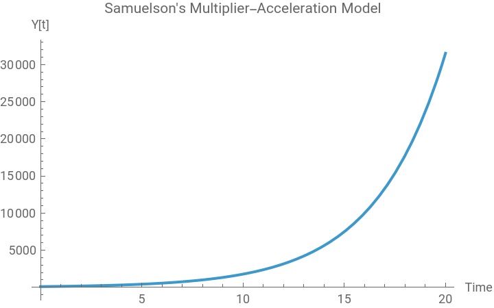
If we assign the following arbitrary values to parameters and the initial value, the aggregate output-income will behave:
In[]:=
ClearAll[α,β,Y,Y0,t,sol];α=0.2;β=0.8;Y0=100;sol=RSolve[{Y[t](-β/(α-β))*Y[t-1],Y[0]==Y0},Y[t],t];Plot[Y[t]/.sol,{t,0,20},PlotLabel->"Samuelson's Multiplier-Acceleration Model",AxesLabel->{"Time","Y[t]"}]
Out[]=
An interactive visualization with varying parameters
An interactive visualization with varying parameters
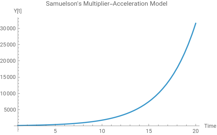
Now suppose the initial value of Y0 =100 is given. We can create the following interactive chart, which shows a highly unstable behavior of aggregate output-income that is affected by parameter values:
In[]:=
ClearAll[α,β,Y,Y0,t];Y0=100;ManipulatePlotY0*,{t,1,20},PlotLabel->"Samuelson's Multiplier-Acceleration Model",AxesLabel->{"Time","Y[t]"},{{α,0.2},0.1,0.25},{{β,0.8},0.4,1.2},SaveDefinitions->True
t
-
β
α-β
Out[]=


The multiplier-acceleration model I
The multiplier-acceleration model I
The acceleration process in response to the variation in aggregate output-income
The acceleration process in response to the variation in aggregate output-income
This time let us introduce the government spending variable. As before, let denote national income at time t, consumption at time t, PBI(t) total private investment spending at time t, and total government expenditure at time t. National income consists of the sum of consumption, private business investment, and government spending. That is, = + PBI(t) + .
Y(t)
C(t)
G(t)
Y(t)
C(t)
G(t)
Suppose that = α where α is the marginal propensity to consume, = β ( - ) where β > 0 represents investment sensitivity to the change in national income, and = G a fixed quantity. With these specifications, let us derive the second-order difference equation for national income implied by these equations.
C(t)
Y(t)
PBI(t)
Y(t-1)
Y(t-2)
G(t)
Substituting both and PBI(t) into AD(t) = and simplifying, we get Y(t) = αY(t) + β (Y(t-1) - Y(t-2)) + G. This becomes β Y(t-2) - βY(t-1) + (1-α)Y(t) = G.
C(t)
Y(t)
This is a second-order non-homogeneous difference equation with constant coefficients. The solution can be found by:
In[]:=
ClearAll[Y,β,α,t,G];RSolve[βY[t-2]-βY[t-1]+(1-α)Y[t]G,Y[t],t]
Out[]=
Y[t]-++
G
-1+α
-t
2
t
--
β
-1+α
β
-4+4α+β
-1+α
1
-t
2
t
-+
β
-1+α
β
-4+4α+β
-1+α
2
A static visualization with fixed parameters and initial values
A static visualization with fixed parameters and initial values
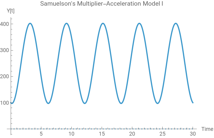
Suppose now that we have the following arbitrary parameters and initial values: α = 0.8, β = 0.4, G = 50. If the two initial values of Y, Y(0) = 100 and Y(1) = 150, then the numerical solution of this equation becomes:
In[]:=
ClearAll[Y,β,α,t,G,sol1];α=0.8;β=0.2;G=50;sol1=RSolve[{βY[t-2]-βY[t-1]+(1-α)Y[t]G,Y[0]==100,Y[1]==150},Y[t],t]
Out[]=
{{Y[t](-75.-14.4338)((-3.21429+0.61859)+(1.+0.)+(0.928571-0.371154))}}
t
(0.5-0.866025)
t
(0.5+0.866025)
In[]:=
ReImPlot[Y[t]/.sol1,{t,0,30},PlotLabel->"Samuelson's Multiplier-Acceleration Model I",AxesLabel->{"Time","Y[t]"}]
Out[]=
The multiplier-acceleration model II
The multiplier-acceleration model II
The acceleration process in response to the variation in household consumption spending
The acceleration process in response to the variation in household consumption spending
We can modify the investment sensitivity slightly. Suppose that = α where α is the output-consumption multiplier, PBI(t) = β( - ) where β > 0 represents investment sensitivity to the change in household consumption measured in two time periods, and = G a fixed government spending.
C(t)
Y(t-1)
C(t)
C(t-1)
G(t)
Since = + PBI(t) + , we get Y(t) = αY(t-1) + β (C(t) - C(t-1)) + G = αY(t-1) + β (α - α) + G. This equation becomes Y(t)- (α +α β) Y[t-1] + α Y[t-2] = G.
Y(t)
C(t)
G(t)
Y(t-1)
Y(t-2)
Notice that this is another linear second-order non-homogeneous difference equation with constant coefficients. The anlytical solution can be found by:
In[]:=
ClearAll[Y,β,α,t,G];RSolve[Y[t]-(α+αβ)Y[t-1]+αY[t-2]==G,Y[t],t]
Out[]=
Y[t]++
G
1-αβ
-t
2
t
α+αβ-
α
-4+α+2αβ+α
2
β
1
-t
2
t
α+αβ+
α
-4+α+2αβ+α
2
β
2
A static visualization with fixed parameters
A static visualization with fixed parameters
Suppose that α = 0.2, β = 0.4, and G = 50. If the two initial values of Y, Y(0) = 100 and Y(1) = 150, then the numerical solution of this equation is:
In[]:=
ClearAll[Y,β,α,t,G,sol2];α=0.8;β=0.2;G=50;sol2=RSolve[{Y[t]-(α+αβ)Y[t-1]+αY[t-2]==G,Y[0]==100,Y[1]==150},Y[t],t]
Out[]=
{{Y[t](20.2381+47.069)((0.458902-1.0673)+(1.+0.)-(0.687947+0.725761))}}
t
(0.48-0.754718)
t
(0.48+0.754718)
In[]:=
ReImPlot[Y[t]/.sol2,{t,0,30},PlotLabel->"Samuelson's Multiplier-Acceleration Model II",AxesLabel->{"Time","Y[t]"}]
Out[]=
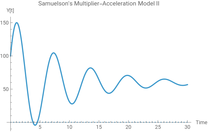
Compared to the first case, the second multiplier-acceleration model seems to converge to its steady state value. This behavior is notwithstanding the same parameter values and the initial condition. Therefore, we can say that the system tends to converge to its steady state value if the private business investment spending responds to the variation in household consumption rather than to the variation in aggregate output-income.
The multiplier-acceleration model with the government sector
The multiplier-acceleration model with the government sector
The model structure and its analytical solution
The model structure and its analytical solution
Now let us extend the previous two models by introducing the government sector’s tax and income transfer. Household consumption will be changed according to its disposable income rather than gross income. As before, let Y(t) denote aggregate output-income at time t, C(t) household consumption at time t, PBI(t) total private business investment spending at time t, and G(t) total government expenditure at time t. National income consists of the sum of household consumption, private business investment spending, and the government spending. That is, AD(t) = Y(t) = C(t) + PBI(t) + G(t).
With these specifications, we can derive the following linear second-order difference equation for national income implied by this specification:
This is a linear second-order non-homogeneous difference equation with constant coefficients. The analytical solution can be found by:
A static visualization with fixed parameters and initial values
A static visualization with fixed parameters and initial values
Suppose that α = 0.2, β = 0.4, τ = 0.2, c0 = 10, TR = 10, and G = 30. If the two initial values of Y are given by Y(0) = 100 and Y(1) = 110, then the numerical solution of this equation becomes:
An interactive visualization with varying parameters
An interactive visualization with varying parameters
We can also create the following interactive chart that enables us to see the changing behavior of the solution curve as the value of some crucial parameters changes:
The accumulation of the capital stock and the government debt
The accumulation of the capital stock and the government debt
The definition of the capital stock and the debt stock
The definition of the capital stock and the debt stock
As the last step, let us think about how to extend previous models with the government sector to account for the capital stock and the government debt accumulation. The private business investment spending will be accumulated as the productive capital stock in the economy. If we assume that there is a constant depreciation rate, δ, the productive capital stock at time t will be:
Similarly, if the sum of the two government spending flows, G + TR, is greater than the government’s tax revenue, τY, the government’s debt will be accumulated as a result of this deficit spending:
Once we determine the initial value of the two variables, K[0] and Debt[0], we can find the analytical solution to each of these two difference equations by:
Notice that both K(t) and Debt(t) are a function of Y(t), which we need to define; once we define the function for Y(t) and then substitute Y(t) into both K(t) and Debt(t), we can find the trajectory of both the capital stock and the debt stock accumulation process.
A static visualization with fixed parameters
A static visualization with fixed parameters
For this purpose, let us continue to use the same parameter values and two initial condition for Y(t) and Y(1) as before: α = 0.8, β = 0.4, τ = 0.2, c0 = 10, TR = 10, G = 30, and Y(0) = 100 and Y(1) = 110 plus δ = 0.02. The numerical solution to Y(t) will remain the same as before. But the two additional solution for K(t) and Debt(t) will be dependent on the solution path of Y(t). The following syntax generates the three solutions.
Interestingly enough, the solution to K(t) is not a single function. Instead, it becomes piecewise function. For visualization purpose, we use ResourceFunction[“EnhancedPlot”] as follow:
An interactive visualization with varying parameters
An interactive visualization with varying parameters
We can also create an interactive chart for the capital stock and debt stock accumulation as follows:
Conclusion
Conclusion
Samuelson’s investment-led business cycle model is one of the greatest contributions made to Keynesian macroeconomics. Samuelson introduced the common sense ideas that the private business investment spending could also adjust to the change in either household consumption and the national income measured at previous time periods. This note demonstrates how we can replicate his core ideas using linear second-order difference equations. We also extended his original model to account for the accumulation of both productive capital stock and the government’s debt stock over time. One can further develop this extended model to account for some labor market variables such as the demand for labor, employment and unemployment, etc., by introducing a fixed capital-labor ratio.
References
References
◼
Alpha C. Chiang, Fundamental Methods of Mathematical Economics, New York: McGraw Hill, 2005, pp.576-581.
◼
Giancharlo Gandolfo, Economic Dynamics, Springer: 2010, pp.73-76.
◼
Michael Hoy, John Livernois, Chris McKenna, Ray Rees, and Thanasia Stengos, Mathematics for Economics, Cambridge, Massachusetts: The MIT Press, 2022 (4th edition), p.809.
◼
Paul Samuelson, “Interaction between the Multiplier Analysis and the Principles of Acceleration.” The Review of Economic Statistics. Vol 20 (1939), pp.75-78.
CITE THIS NOTEBOOK
CITE THIS NOTEBOOK
Introduction to dynamic economic models: Samuelson's investment-acceleration models
by Hee-Young Shin
Wolfram Community, STAFF PICKS, December 24, 2025
https://community.wolfram.com/groups/-/m/t/3596129
by Hee-Young Shin
Wolfram Community, STAFF PICKS, December 24, 2025
https://community.wolfram.com/groups/-/m/t/3596129