In[]:=
$Version
Out[]=
14.0.0 for Microsoft Windows (64-bit) (December 13, 2023)
InverseLaplaceTransform+//TrigToExp,s,t//Simplify(*Undefined???*)
a*Cosh[
s
*y*W0]*u22
a
2
s
Out[]=
Undefined
(*---------------------------------------------------------------------------------------------------------------*)
In[]:=
f[t_]:=InverseLaplaceTransform+/.a->1/.y->1/.W0->1/.u2->1,s,N@t;
a*Cosh[
s
*y*W0]*u22
a
2
s
In[]:=
g[t_,M_]:=NSumu2Hypergeometric1F1-1-2m,,-/.a->1/.y->1/.W0->1/.u2->1,{m,0,M},20;
m
(-1)
1+2m
a
1+2m
t
1
2
2
W0
2
y
4t
Gamma[2+2m]
In[]:=
f[2]
Out[]=
0.663937
In[]:=
g[2,30]
Out[]=
0.66393703293223479042
In[]:=
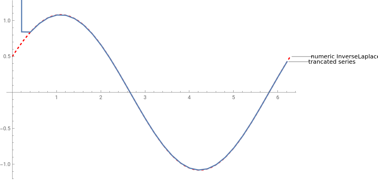
Show[{Plot[g[t,20],{t,0,2*Pi},PlotStyle->{Dashed,Red},PlotLabels"numeric InverseLaplace"],ListLinePlot[Table[{t,f[t]},{t,10^-2,2*Pi,1/5}],PlotLabels"trancated series"]}]
Out[]=