This project investigates the impact of perturbing parameters of a trained neural network on its performance by adding random noise to each layer. My project addresses the big question: “How resilient are neural network to perturbations or noise?”, which has an interesting implication for running neural networks where computational power and resources are limited. In an attempt to answer this question, this experiment observes the performance of a perturbed neural net (LeNet) by adding noise to the pre-trained weights of each layer. As a result of the experiment, this exploratory research has found that a greater magnitude of noise causes severer damage to the performance of the neural network by undermining its capacity to represent the input features. Also, layers responsible for extracting and representing features (e.g., the convolutional layers in LeNet) are particularly more sensitive to perturbations than layers for classification.
1. Introduction
Artificial Neural Networks (ANN) are a type of widely used machine learning model class that is highly successful in a variety of tasks including classification, natural language processing, image processing and etc. A neural network has multiple neurons (linear layer and an non-linear activation function) organized in layers. Each neuron receives input from the previous layer, applies a linear function defined by weights and a bias, applies non-linearity and produce activation or output which is fed into the next layer. The behavior of a neural network model is controlled by its parameters like many other machine learning models. These parameters include the weights that we multiply by an input value and the biases that are added to the weighted sum of the input values. For instance, consider a simple linear layer defined by the following equation: where is the input vector of size , is the scalar output, is the weight vector of size and is the bias termAccording to the definition of dot products, this equation can be also expressed as: Ultimately, these weights determine how much each input value (feature) influences the output of the layer, which could be an activation fed to the next layer or a prediction.Therefore, the objective of a training process is to find the parameters that minimize the loss (or error) and changing the values of the weights significantly influences the model’s prediction and performance. In this light, this computational essay intends to simulate the situation where the weights of a trained model are perturbed with noise. The noise might result from a variety of sources such as lack of computational resources. This research experiments with a pre-trained model, LeNet for image classification and perturbs each individual layer while varying magnitudes of noise.
w
i
x
i
b
a·x+b
T
w
x
n
a
w
n
b
a++...+++b
w
1
x
1
w
2
x
2
w
n-1
x
n-1
w
n
x
n
The LeNet Model
The LeNet Model
LeNet Model is a convolutional neural network for image classification developed by Yann LeCun and his collaborators at AT&T Bell Labs. Trained on the MNIST dataset, it is known to have achieved a significantly high performance in classifying handwritten digits with an error rate less than 1% per digit.
1
In[]:=
leNet=NetModel["LeNet Trained on MNIST Data"]
Out[]=
NetChain


Architecture
Architecture
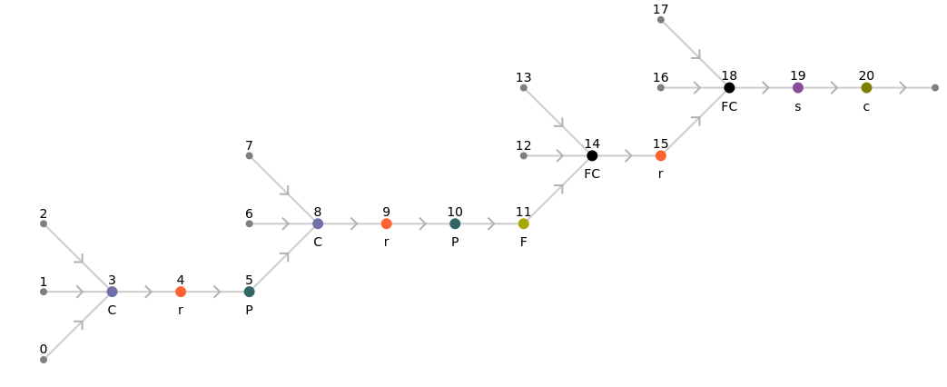
LeNet comprises two main parts: the two convolutional layers and the two fully connected layers. The LeNet takes an image of handwritten digit of size and pass it through the convolutional layers with max pooling to extract its features, which results in a feature map of dimensions . Then, it flattens the feature map into a column vector of size and then pass it through the fully connected layers to classify it. Below are the summary graphics showing the architecture of the LeNet.
2828
5044
1800
In[]:=
Information[leNet,"FullSummaryGraphic"]
Out[]=

In[]:=
Information[NetModel["LeNet Trained on MNIST Data"],"MXNetNodeGraphPlot"]
Out[]=


The MNIST Dataset
The MNIST Dataset
The LeNet is was trained on the MNIST dataset of handwritten digits and is known to have achieved 98.5% accuracy on the MNIST test dataset. The data points are in pairs of image and labels of digits between 0 and 9. The MNIST database consists of a training set of 60,000 examples and a test set of 10,000 examples.
2828
2
In[]:=
mnistTest=ResourceData["MNIST","TestData"];
2. Exploratory Data Analysis: Weight Distribution
Extracting the Weights
Extracting the Weights
We extract the weights from the LeNet for each layer. The 1st (Convolutional), 4th (Convolutional), 8th (Linear) and 10th (Linear) layers have weights.
In[]:=
layerWeights=Table[NetExtract[leNet,{n,"Weights"}],{n,{1,4,8,10}}]
Out[]=
NumericArray,NumericArray,NumericArray
,NumericArray
Summary Statistics
Summary Statistics
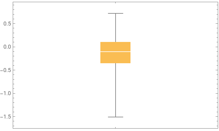
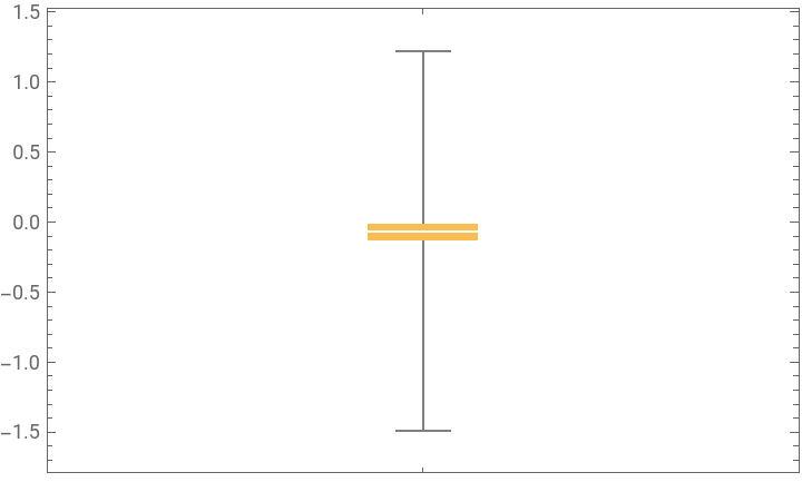
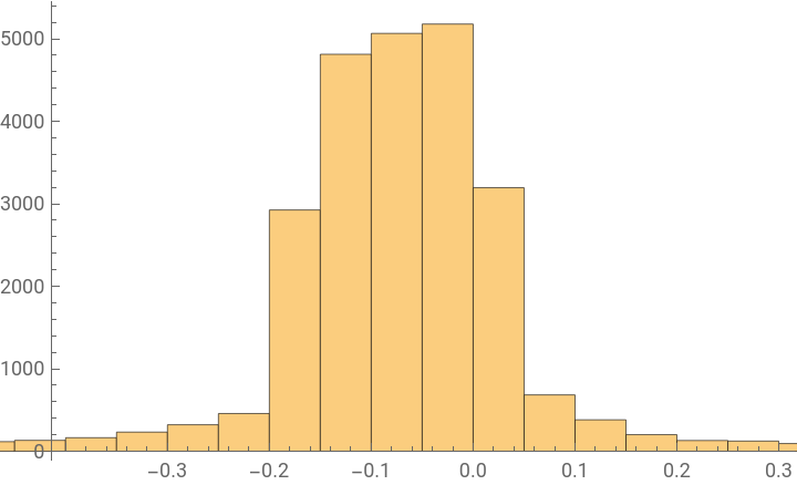
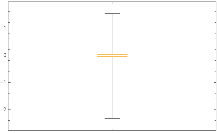
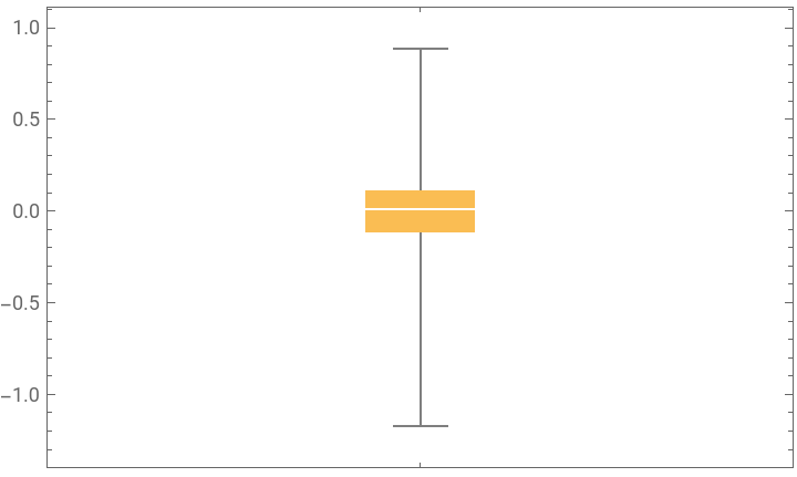
Center: All layers have means and medians close to 0, which indicate that the data centered around zero with slight deviations.
Shape: As we can see from the histograms and the coefficient of skewness, the weight distributions are not symmetrical. Layer 1 (-0.457827) and 4 (-0.463588) are approximately symmetrical but slightly left-skewed shape with moderately small, negatives coefficients of skewness. On the other hand, layer 8 (-1.44888) and 10 (-0.769615) are more left-skewed than the first two with a greater magnitude of skewness coefficient In particular, layer 8 is highly left-skewed with a coefficient significantly less than 1. While the mean and the median of each distribution are fairly close to each other, the mean is slightly less than its median for each distribution. This is likely the result of the slight left skewness, as the extreme values pull the mean to the left side.
Spread: Layer 1 has the highest range (3.87316), which means it has the most variability overall. This is likely influenced by its skewness and the extreme values. The other three layers have fairly similar ranges. Considering the skewness of the distributions, we could use IQR to measure the variability of the data distributions. Layer 1 (0.457827) has the highest IQR, which means it has the greatest central variability.
Graphical Summary
Graphical Summary
We can plot the box plot and histogram of the weights distribution for each layer and visually analyze the center, spread, and shape of the distributions.
In[]:=
Grid[{Style["Weights Distribution",FontSize->20,FontWeight->Bold]},TableForm[Table[{BoxWhiskerChart[Flatten[layerWeights[[l]]//Normal]],Histogram[Flatten[layerWeights[[l]]//Normal]]},{l,1,4}], TableHeadings->{{"Layer 1\n(Convolutional)","Layer 4\n(Convolutional)","Layer 8\n(Linear)","Layer 10\n(Linear)"}}],Spacings->{2,1}]
Out[]=
Weights Distribution | ||||||||||||
|
Numerical Summary
Numerical Summary
The following are the numerical summary of the weights distribution that summarizes the distribution of the weights with numerical measures.
In[]:=
Grid[{{Style["Weights Distribution",FontSize->20,FontWeight->Bold]},{TableForm[Transpose[Table[{Mean[Flatten[layerWeights[[l]]//Normal]],StandardDeviation[Flatten[layerWeights[[l]]//Normal]],Min[Flatten[layerWeights[[l]]//Normal]],Quartiles[Flatten[layerWeights[[l]]//Normal]][[1]],Median[Flatten[layerWeights[[l]]//Normal]],Quartiles[Flatten[layerWeights[[l]]//Normal]][[3]],Max[Flatten[layerWeights[[l]]//Normal]],(Max[Flatten[layerWeights[[l]]//Normal]]-Min[Flatten[layerWeights[[l]]//Normal]]),InterquartileRange[Flatten[layerWeights[[l]]//Normal]],Skewness[Flatten[layerWeights[[l]]//Normal]]},{l,1,4}]],TableHeadings->{{"Mean","Standard Deviation","Min","Q1/4","Median","Q3/4","Max","Range","IQR","Skewness"},{"Layer 1\n(Convolutional)","Layer 4\n(Convolutional)","Layer 8\n(Linear)","Layer 10\n(Linear)"}}]}},Spacings->{2,1}]
3. Method
The four layers in LeNet that have weights are the 1st convolutional layer, the 4th convolutional layer , the 8th linear layer, the 10th linear layer. This experiment assesses the neural network’s sensitivity to perturbations by varying the noise range and the specific layers to which the random noise is added. By randomly sampling noise from various distributions (uniform and Gaussian) and perturbing each layer individually, this experiment aims to identify the most sensitive layer and determine which noise distributions have the greatest impact on the neural network.
Feature Map
Feature Map
Performance Without Noise
Performance Without Noise
The list performanceWithoutNoise contains the test accuracy of the original LeNet and the feature map generated by the convolutional layers, both without adding the noise. This is used to compare the performance of the original neural net with that of the perturbed one.
Noise Range Factor
Noise Range Factor
The list noiseRangeFactor includes the factors by which the range of noise increases. In this experiment, the initial factor is 0.2, and it increments by 0.2 until reaching a final factor of 10. These factors are multiplied by the first and third quartiles and standard deviations to be used as the parameters of the noise distributions.
Noise range for plotting:
Noise from Uniform Distribution
Noise from Uniform Distribution
The first part of this experiment involves adding noise sampled from a uniform distribution to each layer individually. We vary the magnitude of noise added to the weights by varying the range of the noise distribution. The parameters that define a uniform distribution are the minimum and maximum values. In this experiment, we determine the minimum and maximum values in terms of the first and third quartiles and multiply each by a factor between 0.2 and 10 to vary the range.
Noise from Gaussian Distribution
Noise from Gaussian Distribution
The second part of this experiment involves adding noise sampled from a Gaussian distribution to each layer individually. Like in the case of uniform noise distribution, we vary the magnitude of noise added to the weights by varying the range of the noise distribution. The parameters that define a Gaussian distribution are the mean and the standard deviation. In this experiment, we use the mean and the standard deviation of the original weight distribution and multiply each by a factor between 0.2 and 10 to vary the range.
Layer Weights Index
Layer Weights Index
Visualization
Visualization
The function noisePerformancePlot plots the scaling factor on the x-axis and test accuracy for each iteration with a particular scaling factor on the y-axis.
4. Experiment and Results
In this experiment, we add noise sampled from uniform distribution and gaussian distribution to each layer individual. The result is plotted in a 2-D graph with the scaling factor (f) on the x-axis and the test accuracy on the y-axis. The scaling factor determines how great the range of the noise distribution is as we multiply these factors by the standard deviation and quartiles to use as the parameters of the distribution. Therefore, greater scaling factors imply greater magnitude of noise. Then, we compare tendency shown in the layers to each other to infer which layer is more sensitive to perturbations.
Layer 1 (Convolutional Layer)
Layer 1 (Convolutional Layer)
Uniform Distribution
Uniform Distribution
Gaussian Distribution
Gaussian Distribution
Visualization
Visualization
Analysis
Analysis
Layer 4 (Convolutional Layer)
Layer 4 (Convolutional Layer)
Uniform Distribution
Uniform Distribution
Gaussian Distribution
Gaussian Distribution
Visualization
Visualization
Analysis
Analysis
Layer 8 (Linear Layer)
Layer 8 (Linear Layer)
Uniform Distribution
Uniform Distribution
Gaussian Distribution
Gaussian Distribution
Visualization
Visualization
Analysis
Analysis
Layer 10 (Linear Layer)
Layer 10 (Linear Layer)
Uniform Distribution
Uniform Distribution
Gaussian Distribution
Gaussian Distribution
Visualization
Visualization
Analysis
Analysis
The second linear layer has a similar decreasing tendency to the first linear layer although with a slightly faster rate of change. As the noise range increases, the test accuracy gradually decreases. The noise sampled from a Gaussian distribution has a much faster decreasing rate with greater fluctuations.
5. Discussion
For both convolutional and linear layers, greater magnitude of noise decreases the performance of the neural net to a greater extent. However, after having decreased to a certain level of test accuracy (0.2 for the first convolutional layer), the test accuracy levels off as the scaling factor (and therefore, the noise range) increases. Each layer has a different rate of decrease. The perturbation of two convolutional layers causes the neural network to degrade immediately while perturbation of the fully connected layers causes a significantly slower degradation. In other words, layers responsible for feature extraction are more sensitive to the injection of noise while the layers responsible for classification is relatively resilient. This result suggests that when noise is added to the layers for feature extraction (e.g., convolutional layers), the neural network’s ability to extract and represent is impaired.
6. Feature Representation Analysis
Why are the Convolutional Layers much more sensitive and susceptible to perturbations? In an attempt to answer this question, we investigate how the internal feature representation of a Convolutional Neural Network changes as a result of perturbing the weights with noise. A convolutional neural network like LeNet consists of two main parts: convolutional layers and fully connected layers. The main role of convolutional layers is to extract features from the input data for classification by the fully connected layers.
Feature Map
Feature Map
Convolutional Layer 1
Convolutional Layer 1
Convolutional Layer 2
Convolutional Layer 2
Feature Map Example
Feature Map Example
In this section, we observe how the LeNet’s power to represent the features of an image degrades as its weights are perturbed. We take one example from the test dataset of MNIST and feed it to both normal LeNet convolutional layers and the noised one. Then, we compare the visual feature map and observe how feature representation fails as the weights are noised.
Input
Input
Feature Extraction
Feature Extraction
1st Layer (Convolution)
1st Layer (Convolution)
The output of the perturbed first convolutional layer looks visually different from that of the normal one. While the shape of the digit “7” is visible, the color of each feature map is very different.
2nd Layer (ReLU)
2nd Layer (ReLU)
After the output from the first convolutional layer is passed through ReLU, the difference between the perturbed and normal layers becomes clearer. While the feature map of the normal net captures captures the main features like the edges, the feature map of the perturbed net does not at all.
3rd Layer (Pooling)
3rd Layer (Pooling)
4th Layer (Convolution)
4th Layer (Convolution)
5th Layer (ReLU)
5th Layer (ReLU)
6th Layer (Pooling)
6th Layer (Pooling)
The sixth layer is where the final feature map is generated. The feature map from the perturbed net is completely different from that of the normal. We can see that the feature map of the perturbed net does not slightly deviates from the normal one but completely differs, indicating that the neural net has been completely disabled as a result of adding noise.
Classification
Classification
Consequently, fed with contaminated feature map, the fully connected layers misclassify the digit as 1 while it is actually 7.
7th~10th Layer (Fully Connected)
7th~10th Layer (Fully Connected)
7. Conclusion
In this essay, we have investigated how perturbing parameters at different layers influence the performance of a neural network model. As a result of the experiment, we discovered that increasing the magnitude (range) of the noise worsens the performance of the neural network. When the noise is drawn from a Gaussian distribution, the test accuracy fluctuates significantly while decreasing while noise from a Uniform distribution has much less fluctuations. Also, we found out that convolutional layers are considerably more sensitive to noise injection than fully connected layers used for classification since perturbing convolutional layers causes the neural network to degrade immediately. By visualizing and investigating the feature map, we could see noise can completely damage the neural network’s ability to extract and represent features from the input data. On the other hand, the fully connected layer for classification is relatively resilient to noise injection as it caused slow and gradual degradation. This result suggests that perturbing the part of a neural network responsible for feature extracting and representation can severely undermine the predictive power of a neural network.
8. Future Work
This essay about parameter perturbation is primarily concerned with investigating the behavior of a neural network in the presence of noise with little focus on practical application. However, parameter perturbation is highly applicable to real world scenarios where a neural network needs to run on a low-resource environment with limited computational resources or power. Therefore, future works can extend this exploratory research to make conclusions with more significant practical implications. Below are some of the research questions that can help extend this research to practical applications.
1
.Are particular deep learning architectures more sensitive to the injection of noise than others? (e.g., network with multiple convolutional layers vs simple deep network)
2
.How do we make a neural network more resilient to noise perturbations so that they can operate in a low-resource environment?
3
.Would scaling or transforming the weights in a certain way help prevent the neural network from breakdown in the presence of noise?
4
.What computational techniques can be employed to reduce the memory of the weights of a large neural network model to while maintaining functionality?
Acknowledgement
I would like to thank my advisors Jack Heseltime (WSRP Mentor) and Nicolò Monti (WSRP TA) for their guidance and support throughout my project. Additionally, I extend my sincere gratitude to Dr. Stephen Wolfram for providing valuable research ideas and insights.
References
1
.Y. LeCun, L. Bottou, Y. Bengio, P. Haffner, “Gradient-Based Learning Applied to Document Recognition,” Proceedings of the IEEE, 86(11), 2278-2324 (1998)
2
.LeCun, Y., Cortes, C. and Burges, C.J.C. (1998) The MNIST Database of Handwritten Digits. New York, USA. http://yann.lecun.com/exdb/mnist/
3
.Torralba, A., Isola, P., & Freeman, W. T. (2024). Foundations of Computer Vision. The MIT Press.
CITE THIS NOTEBOOK
CITE THIS NOTEBOOK
Impact of parameter perturbation on the neural network performance
by Paul Lee
Wolfram Community, STAFF PICKS, July 11, 2024
https://community.wolfram.com/groups/-/m/t/3217332
by Paul Lee
Wolfram Community, STAFF PICKS, July 11, 2024
https://community.wolfram.com/groups/-/m/t/3217332