Parametric Study of Auto-thermal Gasification of Tunisian Olive Pomace
Housam Binous and Ahmed Bellagi
Parametric Study of Auto-thermal Gasification of Tunisian Olive Pomace
Housam Binous and Ahmed Bellagi
Housam Binous and Ahmed Bellagi
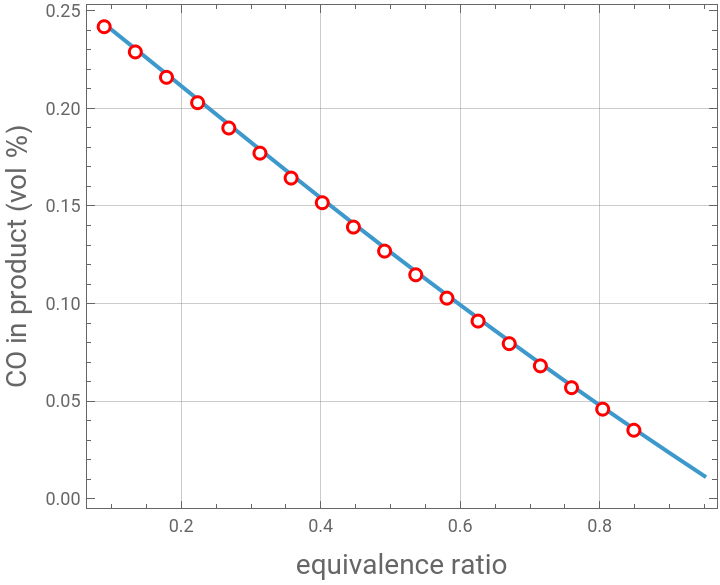
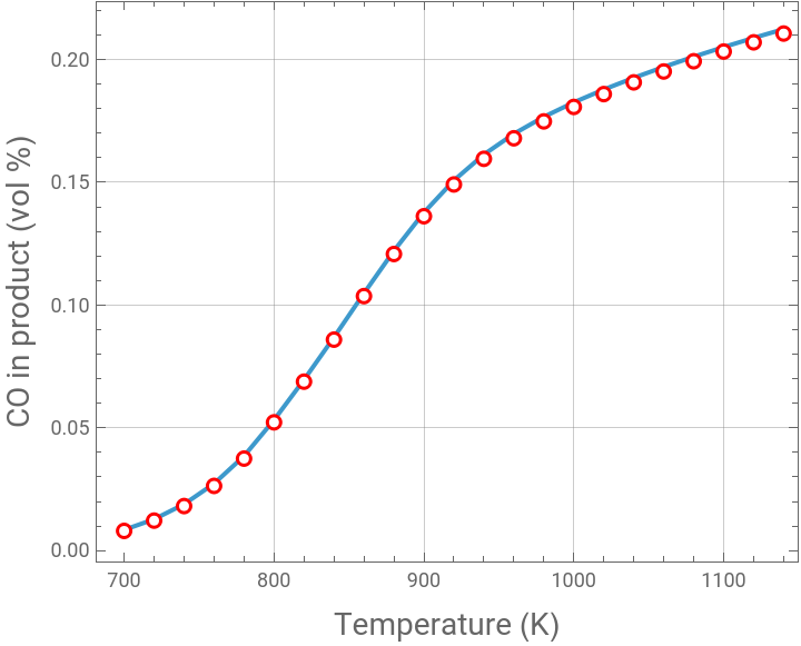
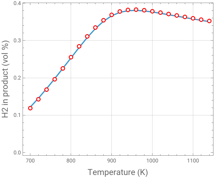
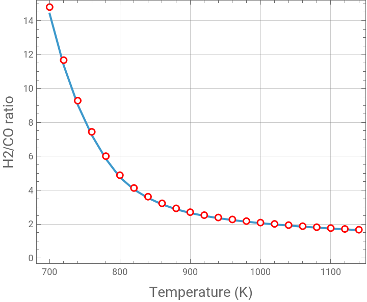
We consider olive pomace gasification (biomass gasification) in the presence of both oxygen and steam (auto-thermal gasification). We assume a constant steam to biomass ratio (S/B) equal to unity. We investigate (1) the effect of temperature for an Equivalence Ratio (ER) equal to 0.3 and the effect of ER when T=1000K.
We present a comparison between our Mathematica calculations and data obtained using Aspen-Plus simulations.
In similar study, presented in Ref. 1, only steam was used as the gasifying agent.
Based on proximate and ultimate analyses, given in Ref. 1, Tunisian olive pomace is modeled as a pseudo-compound whose formula is.
Reference:
[1] R. Tilouche, R. Garma, H. Binous and A. Bellagi, Valorization of Tunisian olive pomace by steam gasification: thermodynamic study using Mathematica© and Aspen-plus®, Biomass Conv. Bioref., 14, 16499–16514 (2024). https://doi.org/10.1007/s13399-023-04167-z
We present a comparison between our Mathematica calculations and data obtained using Aspen-Plus simulations.
In similar study, presented in Ref. 1, only steam was used as the gasifying agent.
Based on proximate and ultimate analyses, given in Ref. 1, Tunisian olive pomace is modeled as a pseudo-compound whose formula is
C
1
H
1.5403
O
0.5318
N
0.0236
Reference:
[1] R. Tilouche, R. Garma, H. Binous and A. Bellagi, Valorization of Tunisian olive pomace by steam gasification: thermodynamic study using Mathematica© and Aspen-plus®, Biomass Conv. Bioref., 14, 16499–16514 (2024). https://doi.org/10.1007/s13399-023-04167-z
In[]:=
In[]:=
sol[x_,ER_,r_]:=Quiet@FindMinimum[{Re[Gtot[x,P]],{n[7]<1/1000000,n[1]>0,n[2]>0,n[3]>0,n[4]>0,n[5]>0,n[6]>0,n[7]>0,n[8]>0,n[9]>0,n[10]>0},n[1]+n[5]+n[4]+n[10]1,4n[1]+2n[2]+2n[3]1.5403+2r,n[3]+n[4]+2n[5]+n[6]+2n[7]+2n[9]0.531858+r+2ER1.119146,n[6]+n[7]+2n[8]0.0236745},Table[{n[j],0.07},{j,1,10}],MaxIterations10000,AccuracyGoal5];
Effect of temperature for an ER = 0.3 and S/B ratio = 1
In[]:=
P=1;
In[]:=
tbl=Table[{T,y[4]/.sol[T,0.3,1.0][[2]]},{T,700,1150,20}];
In[]:=
p1=ListPlot[tbl,PlotRange->All,Frame->True,AspectRatio->0.8,GridLines->Automatic,Joined->True,FrameLabel->{Style["Temperature (K)",14],Style["CO in product (vol %)",14]}];
In[]:=
(*ASPEN*)tbl2={{700,0.00802472443},{720,0.0122151808},{740,0.0181468554},{760,0.0263562016},{780,0.0374783234},{800,0.0522408995},{820,0.06881811},{840,0.0859270904},{860,0.10366245},{880,0.120800101},{900,0.136190408},{920,0.149132809},{940,0.159570636},{960,0.167938178},{980,0.174819992},{1000,0.180708226},{1020,0.185936835},{1040,0.190709817},{1060,0.195146845},{1080,0.199318208},{1100,0.203266477},{1120,0.207018852},{1140,0.210593956}};
In[]:=
p2=ListPlot[tbl2,PlotMarkers->"OpenMarkers",PlotStyle->Red];(*Aspenresultsarerepresentedusingredopenmarkers*)
In[]:=
Show[p1,p2]
Out[]=
In[]:=
tbl=Table[{T,y[2]/.sol[T,0.3,1.0][[2]]},{T,700,1150,20}];
In[]:=
p1=ListPlot[tbl,PlotRange->All,Frame->True,AspectRatio->0.8,GridLines->Automatic,Joined->True,FrameLabel->{Style["Temperature (K)",14],Style["H2 in product (vol %)",14]}];
In[]:=
(*ASPEN*)tbl2={{700,0.118734197},{720,0.142533628},{740,0.168429813},{760,0.19611185},{780,0.225217464},{800,0.25535744},{820,0.28445381},{840,0.311115799},{860,0.334842749},{880,0.354379998},{900,0.368778695},{920,0.377792087},{940,0.382049277},{960,0.38276347},{980,0.381203458},{1000,0.378350019},{1020,0.374838374},{1040,0.371040765},{1060,0.367163809},{1080,0.363318609},{1100,0.359563258},{1120,0.355926828},{1140,0.352422524}};
In[]:=
p2=ListPlot[tbl2,PlotMarkers->"OpenMarkers",PlotStyle->Red];(*Aspenresultsarerepresentedusingredopenmarkers*)
In[]:=
Show[p1,p2]
Out[]=
In[]:=
tbl=Table[{T,y[2]/y[4]/.sol[T,0.3,1.0][[2]]},{T,700,1150,20}];
In[]:=
p1=ListPlot[tbl,PlotRange->All,Frame->True,AspectRatio->0.8,GridLines->Automatic,Joined->True,FrameLabel->{Style["Temperature (K)",14],Style["H2/CO ratio",14]}];
In[]:=
tbl2={{700,14.7960467},{720,11.6685647},{740,9.28148756},{760,7.44082372},{780,6.00927264},{800,4.88807509},{820,4.13341502},{840,3.62069514},{860,3.23012576},{880,2.9336068},{900,2.70781695},{920,2.53325938},{940,2.39423296},{960,2.2791927},{980,2.18054843},{1000,2.09370667},{1020,2.01594468},{1040,1.94557769},{1060,1.88147448},{1080,1.82280692},{1100,1.76892552},{1120,1.7192967},{1140,1.67346932}};(*ASPEN*)
In[]:=
p2=ListPlot[tbl2,PlotMarkers->"OpenMarkers",PlotStyle->Red];(*Aspenresultsarerepresentedusingredopenmarkers*)
In[]:=
Show[p1,p2]
Out[]=
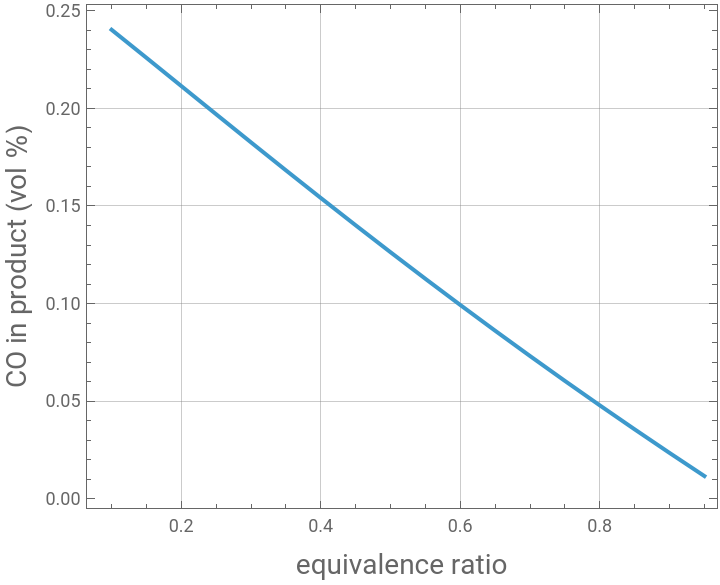
Effect of ER for temperature = 1000 K and S/B ratio = 1
In[]:=
P=1;
In[]:=
tbl=Table[{ER,y[4]/.sol[1000,ER,1.0][[2]]},{ER,0.1,0.95,0.05}]
Out[]=
{{0.1,0.240287},{0.15,0.225915},{0.2,0.211449},{0.25,0.196978},{0.3,0.182566},{0.35,0.168262},{0.4,0.154099},{0.45,0.140103},{0.5,0.126292},{0.55,0.11268},{0.6,0.0992768},{0.65,0.0860896},{0.7,0.0731226},{0.75,0.0603784},{0.8,0.0478584},{0.85,0.0355622},{0.9,0.0234888},{0.95,0.0116356}}
In[]:=
p1=ListPlot[tbl,PlotRange->All,Frame->True,AspectRatio->0.8,GridLines->Automatic,Joined->True,FrameLabel->{Style["equivalence ratio",14],Style["CO in product (vol %)",14]}]
Out[]=
In[]:=
(*ASPEN*)tbl2={{0.1,0.24184763},{0.15,0.228929646},{0.2,0.215928887},{0.25,0.202918475},{0.3,0.189952151},{0.35,0.177069883},{0.4,0.164301671},{0.45,0.151670159},{0.5,0.139192471},{0.55,0.126881505},{0.6,0.114746879},{0.65,0.102795626},{0.7,0.0910327135},{0.75,0.0794614431},{0.8,0.0680837569},{0.85,0.056900482},{0.9,0.0459115244},{0.95,0.0351160262}};(*abscissaismolarflowofO2*)
In[]:=
tbl2=Table[{tbl2[[i]][[1]]/1.119146,tbl2[[i]][[2]]},{i,1,Length@tbl2}];(*abscissaisER*)
In[]:=
p2=ListPlot[tbl2,PlotMarkers->"OpenMarkers",PlotStyle->Red];(*Aspenresultsarerepresentedusingredopenmarkers*)
In[]:=
Show[p1,p2]
Out[]=