Determining the behavior of a Cellular Automaton from a designated rule is straightforward, but inverse designing CA rules so that they exhibit a desired behavior is much more complex and interesting to study. Many previous works have used algorithms such as genetic algorithms and randomized hill climber to generate CA rules(Mitchell et al., 1996). In this essay, I specifically explore how Simulated Annealing can generate CA rules that behave in desired ways. Some classes of rules I explore include Binary Totalistic Probabilistic CA and 3-state Deterministic CA. I compare SA’s ability to find rules that live for a desired lifetime to the ability of other standard algorithms. I also explore the impact of different cooling schedules and step sizes on SA’s effectiveness. Future work should focus on expanding the tasks for CA and analyzing SA performance against more diverse approaches such as genetic algorithms.
Introduction
Introduction
Cellular automata are models consisting of grids whose states evolve over discrete time steps according to a rule. There are many different families of CA rules. A few that I focus on are Totalistic versus General rules, along with Probabilistic versus Deterministic rules.
Totalistic rules only take into consideration the sum of the states of the cells in the neighborhood of the current cell, while General rules determine the next cell value depending on the specific configuration of the cells in its neighborhood.
Probabilistic rules assign a cell value based on a probability for each state of the neighborhood, so the result of each evaluation of a probabilistic rule can be different. Deterministic rules assign the cell a value for each configuration, producing the same result for all evaluations with the same initial condition.
The algorithm I am studying is Simulated Annealing, or SA, a randomized optimization algorithm that finds an optimal or near optimal solution by escaping local minima with a decreasing temperature parameter. The two algorithms I compared SA to are Randomized enumeration and Randomized Hill Climber. Randomized Enumeration samples n random rules, where n is the number of iterations used by the SA algorithm in the comparison, and returns the rule with the lowest loss; randomized Hill Climber is the more naive algorithm similar to SA but doesn’t involve the decreasing temperature parameter and behaves greedily on every iteration.
For simplicity and for a fairer performance comparison, the target behavior I evolve the rule for is CA lifetime. For a Deterministic CA, the loss function I minimize is the difference between the number of steps it takes the CA rule to reach the all-zeros state and the target lifetime. For Probabilistic automata, the loss function is the difference between the target lifetime and the average number of steps it takes the rule to reach the all-zeros state over many trials; the accuracy of this estimate increases as the number of trials increases.
The results showed that SA outperforms randomized hill climber and randomized enumeration in complex rule spaces, most noticeably when searching for relatively small target lifetime. This is most likely a result of SA’s superior ability to escape local minima on complex rule spaces. SA performs at similar level as hill climber and enumeration when the rule space is too simple, too discrete, or when the target lifetime is relatively large, resulting in less clustered rules and local minima, thus less need for the ability to escape regional optimality.
General Simulated Annealing
General Simulated Annealing
Simulated Annealing is a probabilistic optimization algorithm used to find best or near-best solutions for complex problems. Its name comes from the metallurgical concept of annealing, in which a material is heated and cooled according to a cooling schedule in order to alter the material’s properties. SA has a temperature parameter that controls how likely the algorithm is to choose a candidate solution that is worse than the current one. This strategy allows it to escape local minima.
For example, one application of SA is the traveling salesman problem. A Randomized Hill Climber may get stuck on a route that is better than all routes reachable by a small local change, even though that route is still worse than the globally optimal route. SA can escape this kind of local minimum by making bolder jumps at high temperatures. As the temperature decreases, SA becomes more selective and refines its answer within the most promising region.
SA for Finding a Global Minimum
SA for Finding a Global Minimum
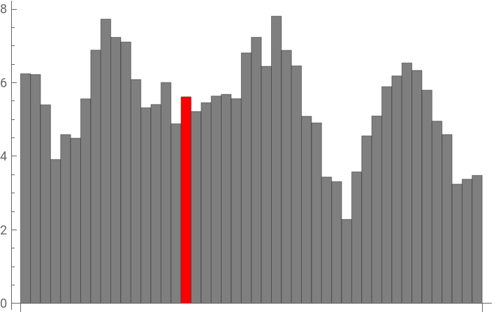
Below is an example of using SA to find the minimum value of a random function that consists of many local minima.
Using SA on this problem does not have much practicality because the problem is discrete and simply enumerating the values would be efficient enough. However, it serves as a useful visual demonstration for understanding the properties of SA .
Using SA on this problem does not have much practicality because the problem is discrete and simply enumerating the values would be efficient enough. However, it serves as a useful visual demonstration for understanding the properties of SA .
First I generate a random array:
In[]:=
arr=MovingAverage[RandomReal[{0,10},50],5];
In[]:=
makeFr[sp_]:=Graphics[BarChart[arr,ChartStyle->ReplacePart[ConstantArray[Gray,Length[arr]],sp->Red]]]
In[]:=
Length[arr]
Out[]=
46
Set the temperature and step size:
In[]:=
saIter=500;len=46
Out[]=
46
In[]:=
sTmp=5.;eTmp=0.05;
In[]:=
sStep=15;eStep=1;
The first rule proposing function follows a gaussian distribution and use step sizes that are potentially out of the set boundary:
In[]:=
propRule1[cur_,step_]:=Clip[cur+Round[RandomVariate[NormalDistribution[0,step]]],{1,len}]
The second rule proposing function use step sizes strictly within the set boundary:
In[]:=
propRule2[cur_,step_]:=Clip[cur+RandomInteger[{-step,step}],{1,len}]
In[]:=
cur=RandomInteger[{1,len}]curEr=arr[[cur]]
Out[]=
43
Out[]=
3.72333
In[]:=
best=cur;bestE=curEr;
Three types of cooling schedules; explained in the next section:
In[]:=
sched[i_Integer,n_Integer,start_,finish_,typ_:1]:=Module[{u},u=(i-1)/(n-1);Which[typ==1,start*(finish/start)^u,typ==2,start+(finish-start)*u,typ==3,start+(finish-start)*u^2]];
The red bar represents the current best solution the algorithm has found:
cur=RandomInteger[{1,len}];curEr=arr[[cur]];best=cur;bestE=curEr;tmpList={};stepList={};
Clear[fr]fr=Reap[Monitor[curEgraph=Reap[Table[tmp=sched[iter,saIter,sTmp,eTmp,1];step=Round[sched[iter,saIter,sStep,eStep,2]];AppendTo[tmpList,tmp];AppendTo[stepList,step];cand=propRule2[cur,step];candEr=arr[[cand]];delta=candEr-curEr;ac=delta<=0||RandomReal[]<Exp[-delta/tmp];If[ac,cur=cand;curEr=candEr;];If[curEr<bestE,best=cur;bestE=curEr;Sow[makeFr[best]]];,{iter,Range[1,saIter]}];][[2]],iter]][[1]];
ListAnimate[Flatten[fr]]
Out[]=
Cooling Schedules
Cooling Schedules
The simulation above was generated with SA using a geometric cooling schedule, which is one of the three cooling schedules I explore.
In geometric cooling, the temperature decreases quickly at first and becomes more constant toward the end. The benefit of geometric cooling is that the solution has a longer phase of low temperature at the end. Because the algorithm is likely exploring the small region it has already identified as optimal toward the end, a consistently low temperature allows it to search that region in a greedy-like manner and find a better minimum.
In geometric cooling, the temperature decreases quickly at first and becomes more constant toward the end. The benefit of geometric cooling is that the solution has a longer phase of low temperature at the end. Because the algorithm is likely exploring the small region it has already identified as optimal toward the end, a consistently low temperature allows it to search that region in a greedy-like manner and find a better minimum.
Create plot for all three types of cooling schedules:
tmpListG={};tmpListL={};stepListG={};stepListL={};tmpListA={};stepListA={};
Monitor[Table[tmpG=sched[iter,saIter,sTmp,eTmp,1];tmpL=sched[iter,saIter,sTmp,eTmp,2];stepG=Round[sched[iter,saIter,sStep,eStep,1]];stepL=Round[sched[iter,saIter,sStep,eStep,2]];tmpA=sched[iter,saIter,sTmp,eTmp,3];stepA=Round[sched[iter,saIter,sStep,eStep,3]];AppendTo[tmpListG,tmpG];AppendTo[tmpListL,tmpL];AppendTo[stepListG,stepG];AppendTo[stepListL,stepL];AppendTo[tmpListA,tmpA];AppendTo[stepListA,stepA];,{iter,Range[1,saIter]}],iter];
Another possible cooling schedule is linear cooling, where the temperature decreases steadily as the algorithm iterates. The benefit of a linear cooling schedule is that it gives each phase enough iterations so that the algorithm can jump out of broad basins of local minima while still having enough time to refine smaller local choices within the region containing the global minimum.
The final cooling schedule is accelerated cooling. In accelerated cooling, the rate of temperature decrease increases over iterations, essentially producing the opposite effect of geometric cooling. Accelerated cooling gives the high - randomization phase more iterations and may be useful for data that contains many regions of possible global minimality but does not contain many local minima within the region of the global minimum .
In the global minimum example, the starting temperature was 15 and the ending temperature was 0. The ending temperature of SA is usually very close to 0 in order to ensure that the algorithm can refine its solution through a greedy like search after locating the correct region. Increasing the starting temperature makes the algorithm more explorative in the beginning and is better for problems with very complex solution spaces, while a lower starting temperature allows SA to focus on specific regions more quickly.
Changing the starting temperature:
Graph of the value of the current loss function for each evaluation:
Lower starting temperature:
Graph of the value of the current loss function for each evaluation:
As seen on the two graphs, I can see that the algorithm accepts worse solution more boldly when the temperature is higher.
Step Sizes
Step Sizes
The other SA parameter I explore is step size, which determines how far each randomly proposed candidate rule should be from the current rule. Most SA implementations have either a constant or decreasing step size. In my CA project, I use a decreasing step size so that the algorithm can explore the general rule space through large jumps at first and then further explore a promising region after it has been located. During the later phase, smaller step sizes let the algorithm fine-tune its solution within the general region. This is especially helpful for probabilistic CA rules, where the rule parameters are continuous but the resulting CA behavior may change in irregular, non-continuous ways.
In the SA global minimum example above, I used a linearly decreasing step size. The graph appears discrete because step sizes are rounded for this example; this will not be the case for probabilistic CA rules.
In the SA global minimum example above, I used a linearly decreasing step size. The graph appears discrete because step sizes are rounded for this example; this will not be the case for probabilistic CA rules.
Creating graph for step size for each evaluation when using linearly decreasing step size:
Creating graph for step size for each evaluation when using geometrically decreasing step size:
Creating graph for step size for each evaluation when using accelerating decreasing step size:
Binary Probabilistic Totalistic Cellular Automata
Binary Probabilistic Totalistic Cellular Automata
The first CA rule family I am testing is Binary Totalistic Probabilistic CA, which considers the sum of the states of the cells in the neighborhood without regard for the exact configuration, and assigns the cell a state based on a probability parameter for each sum.
I set the maximum number of rows the CA is allowed to live for and initialize the first row to have a singular 1 surrounded by 0’s:
Below is an assignment of probabilities for each possible neighborhood sum; when its neighborhood sum to 0, the probability of the cell being 1 is 0, when the sum is 1, the probability is 0.4, etc:
Example CA:
Because our loss function is concerning the lifetime of the CA rule, I hereby define the lifetime of a rule set as the average time it takes for multiple runs using this same rule to reach a state of all zeros. The exact number of runs I am averaging will vary depending on the efficiency of each of the algorithms, in order to give each algorithm equal resources when computing and help make comparisons between their performances.
Because of the uncertainty involved in using Probabilistic CAs, faster lifetime evaluation will allow more runs for a more accurate average.
To achieve this, I attempted three methods of assessing average lifetime of a CA rule, finding the third to be the most efficient.
Our first attempt at a function finding the average lifetime of a CA rule is based on the Wolfram Language’s system CellularAutomaton function. However, this implementation required us to use an association to represent the probabilities for each of the possible neighborhood sums and could not end the evaluation before reaching the designated max number of iterations, even if the Cellular Automata already had a state of all 0.
Finding time of death of a CA rule using Wolfram system function:
Our second attempt involved the Wolfram Resource Repository Function ProbabilisticCellularAutomaton, which shortened the algorithm, but did not see enough of an increase in evaluation speed. Most importantly, ProbabilisticCellularAutomaton is primarily for General CA rules instead of Totalistic, but for reference I still included an example implementation below.
Finding time of death of a General CA using Wolfram Resource Repository Function:
In our final attempt, I steered towards more procedural programming for more classic optimization techniques, which, although involved several nested For loops, was able to most efficiently evaluate entire rows simultaneously and stop the computation as soon as all cells turn to blank. Because I basically recreated the entire CellularAutomaton function, compiling the function all to C also was able to drastically speed up the processing time of the procedural program. The reader can add in the CompilationTarget -> “C” option on their local notebook if needed.
Most efficient implementation of building the CA from the ground up with procedural programming:
Performance on Binary Totalistic Probabilistic Cellular Automaton With Radius 1
Performance on Binary Totalistic Probabilistic Cellular Automaton With Radius 1
First I assess SA’s performance on Binary Totalistic Probabilistic Cellular Automata with Neighborhood radius of 1, meaning I only consider the sum of the states of each cell’s two immediate neighbors and itself.
I start with three random probabilities. SA and the two standard algorithms I am testing it against will then use their respective methods to evolve the rules so that the average lifetime of the CA is as close as possible to the target lifetime.
Performance is measured by running each algorithm 50 times and finding the mean and standard deviation of each of the results. The better performing algorithm will have mean closer to the desired target and a smaller standard deviation.
Simulated Annealing with target lifetime 25
Simulated Annealing with target lifetime 25
Different cooling schedules and step size schedules are already discussed in the General Simulated Annealing section, so additional tests for all configurations of cooling schedules and step size schedules tested would make the essay unnecessarily long. The code below uses geometric schedule for both temperature and step size, which is the configuration that produced the best results in testing.
To better visualize the process through which SA search for optimal rules, the rule space I am searching through can be viewed as a three-dimensional box with side length 1.
The x, y, z coordinates represent the probabilities of a cell being 1 when its neighborhood sums to 1, 2, and 3, respectively.
Set number of trials to average between and target lifetime to search for, and how many times SA should iterate:
Set starting and ending temperature and step size:
The first rule proposing function follows a gaussian distribution and use step sizes that are potentially out of the set boundary:
The second rule proposing function use step sizes strictly within the set boundary:
Color and frame making for the animation:
The animation below shows the process of SA exploring the rule space; smaller spheres are explored rules and large spheres are accepted rules, their color represent how close the rule is to target lifetime, with better rules appearing redder:
Now I run SA 50 times with target lifetime 25:
I visualize SA’s search process as a graph of the loss function with respect to iterations. The graph below is for the 50th SA run:
I evaluate the average lifetime of each of the rules SA found:
Over 50 independent SA runs for the target lifetime of 25, I found the mean of the 50 average lifetimes of the rules to be 25.381, which is close to our target of 25, indicating a high accuracy. The standard deviation of the results was 1.381, indicating that the algorithm consistently had high performances across runs.
Randomized Hill climber with target lifetime 25
Randomized Hill climber with target lifetime 25
The randomized Hill climber has a process similar to SA, except it does not have the temperature parameter. During every iteration, Hill Climber will only behave greedily and accept changes that decrease the loss.
I graph hill climber’s loss against its iterations for the 50th run:
Hill Climber never accepts changes that make the rule worse, so the loss function is strictly non increasing.
I evaluate the average lifetime of each of the rules Hill Climber found:
Over 50 independent Hill Climber runs for the target lifetime of 25, I found the mean of the 50 average lifetimes of the rules to be 25.273, which is close to our target of 25, indicating a high accuracy. The standard deviation of the results was 2.067, indicating that the algorithm consistently had relatively high performances across runs.
Randomized Enumeration with target lifetime 25
Randomized Enumeration with target lifetime 25
The Randomized Enumeration is the most naive algorithm. It simply enumerates random independent rules and takes the optimal one.
One thing to note is that because the target lifetime is only 25, both SA and Hill Climber will quickly narrow down their search space to only explore rules that have a relatively small lifetime. Enumeration, however, will be randomly generating independent rules, meaning it will be testing many rules that have a much larger average lifetime, which takes significantly longer time to evaluate. To make the comparison fair by giving all three algorithms equal computing power, I decreased the number of iterations Enumeration performs from 300 down to 100, which gave it an average runtime of slightly longer than the average runtime of SA, providing a fair comparison.
One thing to note is that because the target lifetime is only 25, both SA and Hill Climber will quickly narrow down their search space to only explore rules that have a relatively small lifetime. Enumeration, however, will be randomly generating independent rules, meaning it will be testing many rules that have a much larger average lifetime, which takes significantly longer time to evaluate. To make the comparison fair by giving all three algorithms equal computing power, I decreased the number of iterations Enumeration performs from 300 down to 100, which gave it an average runtime of slightly longer than the average runtime of SA, providing a fair comparison.
I evaluate the average lifetime of each of the rules the enumeration found:
Over 50 independent enumeration runs for the target lifetime of 25, I found the mean of the 50 average lifetimes of the rules to be 24.135 which is slightly farther off our target of 25, indicating a relatively lower accuracy. The standard deviation of the results was 5.197, indicating that the algorithm had relatively more inconsistent performances across runs .
Comparison
Comparison
Out of the three algorithms, SA and Hill Climber had similar performances, with SA having slightly higher precision and Hill Climber having a slightly higher accuracy. enumeration had a slightly worse performance. Overall, the difference was not significant enough for me to definitely conclude whether SA generally performs better or worse than Hill Climber or enumeration.
Performance on Binary Totalistic Probabilistic Cellular Automaton With Radius 2
Performance on Binary Totalistic Probabilistic Cellular Automaton With Radius 2
Now I assess SA's performance on Binary Totalistic Probabilistic Cellular Automata with Neighborhood radius of 2, meaning I only consider the sum of the states of each cell's four neighbors and itself.
I start with five random probabilities.
Performance is measured by the running each algorithm 50 times and finding the mean and standard deviation of each of the results .
I start with five random probabilities.
Performance is measured by the running each algorithm 50 times and finding the mean and standard deviation of each of the results .
First I modify the earlier deathTime function to adapt to CA with neighborhood size of five:
Simulated Annealing with target lifetime 25
Simulated Annealing with target lifetime 25
Set target lifetime, iterations, starting and ending temperature and step size:
Two rule proposal strategies are the same as before, except now adapted for neighborhood of 5 cells:
Run SA:
Find the actual death time by averaging 10000 runs:
Plot the loss as a function of iterations for SA:
Now I run SA 50 times:
Evaluate the average lifetime of each of the rules SA found:
Over 50 independent SA runs for the target lifetime of 25, I found the mean of the 50 average lifetimes of the rules to be 25.394 which is close to the target, indicating a high accuracy. The standard deviation of the results was 1.606, indicating that the algorithm had consistent performances across runs .
Randomized Hill Climber with Target lifetime 25
Randomized Hill Climber with Target lifetime 25
I run the hill climber modified for neighborhood size of 5:
Plot hill climber’s loss for each iteration:
Run hill climber 50 times:
Find the average lifetime of each of the rules hill climber found:
Over 50 independent hill climber runs for the target lifetime of 25, I found the mean of the 50 average lifetimes of the rules to be 26.435, which is significantly farther from target than the previous algorithm, indicating low accuracy. The standard deviation of the results was 12.567, indicating that the algorithm had very inconsistent performances across runs .
Randomized Enumeration with target lifetime 25
Randomized Enumeration with target lifetime 25
The enumeration is also adapted for neighborhood size of 5:
Run enumeration 50 times:
Evaluate the average lifetime of each of the rules the enumeration found .
Over 50 independent enumeration runs for the target lifetime of 25, I found the mean of the 50 average lifetimes of the rules to be 24.81, which is close to target, indicating a high accuracy. The standard deviation of the results was 8.548, indicating that the algorithm had very inconsistent performances across runs .
Simulated Annealing with target lifetime 250
Simulated Annealing with target lifetime 250
Run SA 50 times for target of 250:
Evaluate the average lifetime of each of the rules SA found:
Over 50 independent SA runs for the target lifetime of 250, I found the mean of the 50 average lifetimes of the rules to be 249.387, which is very close to target, indicating a high accuracy. The standard deviation of the results was 28.223, indicating that the algorithm had very inconsistent performances across runs .
Randomized Hill Climber with Target lifetime 250
Randomized Hill Climber with Target lifetime 250
Run hill climber 50 times for target of 250:
Evaluate the average lifetime for each of the rules found:
Over 50 independent hill climber runs for the target lifetime of 250, I found the mean of the 50 average lifetimes of the rules to be 253.317, which is close to target, indicating a high accuracy. The standard deviation of the results was 25.624, indicating that the algorithm had inconsistent performances across runs .
Randomized Enumeration with target lifetime 250
Randomized Enumeration with target lifetime 250
Run Enumeration 50 times for target lifetime of 250:
Evaluate the average lifetimes of the rules found:
Over 50 independent enumeration runs for the target lifetime of 250, I found the mean of the 50 average lifetimes of the rules to be 257.386, which is moderately far from target, indicating a relatively low accuracy. The standard deviation of the results was 24.704, indicating that the algorithm had inconsistent performances across runs .
Comparison
Comparison
For binary probabilistic totalistic CA rules with neighborhood size of 5, I tested each of the three algorithms on a target lifetime of 25 and 250. SA vastly outperformed the other two algorithms when the target lifetime was small, having a negligible difference in mean and significantly lower standard deviation. For a target lifetime of 250, SA had the closest mean to the target but also the highest standard deviation. However, the difference is not significant enough to conclude any general performance difference.
Performance on 3 State General Cellular Automata With Radius 1
Performance on 3 State General Cellular Automata With Radius 1
First I adapt the earlier death time function for general CA:
Simulated Annealing with target lifetime 250
Simulated Annealing with target lifetime 250
Now I modify SA for general CA. step sizes are now represented with mutation counts, which represent how many bits of the rule table to flip at one time. I also needed to add additional functions to help convert between rule tables and rule numbers.
Initializing target lifetime, iterations, temperature, and mutation counts:
The function for proposing new rules.
Evaluating rules by first converting from rule table to rule number:
Run SA once:
Evaluate the real lifetime:
Visualize what the rule SA found looks like, and confirm the lifetime:
Plot SA loss against iterations:
Because of the high iteration counts, the small rises in loss function caused by the high temperature in the beginning is much less visible than the previous SA runs.
Run SA 50 times:
Evaluate the lifetime of the 50 rules found:
Over 50 independent SA runs for the target lifetime of 250, I found the mean of the 50 average lifetimes of the rules to be 194.44, which is far from target, indicating a low accuracy. The standard deviation of the results was 76.999, indicating that the algorithm had very inconsistent performances across runs .
Randomized Hill climber with target lifetime 250
Randomized Hill climber with target lifetime 250
Run the hill climber adapted for general CA:
Evaluate the real lifetime of the rule hill climber found:
Without a temperature parameter, hill climber’s loss function is strictly non increasing.
Run hill climber 50 times:
Evaluate the average lifetime of the rules found:
Over 50 independent hill climber runs for the target lifetime of 250, I found the mean of the 50 average lifetimes of the rules to be 226.8, which is relatively close to target, indicating a high accuracy. The standard deviation of the results was 68.796, indicating that the algorithm had very inconsistent performances across runs .
Randomized Enumeration with target lifetime 250
Randomized Enumeration with target lifetime 250
Run the enumeration adapted for general CA:
Evaluate the real lifetime of the rule found:
Run enumeration 50 times:
Evaluate the lifetime of each of the rules found:
Over 50 independent enumeration runs for the target lifetime of 250, I found the mean of the 50 average lifetimes of the rules to be 31.32, which is extremely far from target, indicating a very low accuracy. The standard deviation of the results was 46.030, indicating that the algorithm had very inconsistent performances across runs.
Discussion
Discussion
Across all three of the rule spaces tested, SA had performances that were sometimes superior and sometimes comparable to traditional algorithms such as randomized hill climber and randomized enumeration. However, SA did not consistently outperform them in all rule spaces.
Most notably, SA performed significantly better than traditional algorithms for Probabilistic Totalistic CA with neighborhood size of 5, with the most visible difference when the target lifetime is smaller.
For Probabilistic Totalistic CA with neighborhood size of 3, the rule space was a simple 3 dimensional box. The lack of sufficient complexity and local optimality reduced the need for SA’s ability to find global minimum in complex landscapes, and resulted in a performance that was not significantly better than a greedy hill climber search or random enumeration.
For Probabilistic Totalistic CA with neighborhood size of 5, the rule space was sufficiently complex. However, due to the tendency of Totalistic CA to have an infinite lifetime, rules that result in a small average lifetime are much more clustered than rules that result in a larger, but still finite average lifetime. This means that the rule space for smaller lifetimes will be more complex and naturally giving more use to SA’s ability to escape local minima. But this landscape is much simpler and smoother for greater average lifetime because most rules either die out very soon or live on forever. This simple landscape causes SA to perform trivially, and sometimes even inferior to traditional algorithms; the latter is because SA wastes many early iterations accepting rule changes that increase loss, but doesn’t escape any local minimality.
For Deterministic CA, the situation is more interesting. Initially I was expecting both SA and hill climber to produce results no better than randomized enumeration, because the rule space appears to be completely discrete, with small bit flips resulting in drastic behavioral changes. However, I soon discovered that was not the case. Taking a closer look at the fitness landscape of 3 state deterministic general CA with neighborhood size of 3 revealed that, even though most of the rules had an infinite lifetime and the rules having a finite lifetime appear randomly, if I remove all the rules with an infinite lifetime, or those that lives past a threshold which I used 7000, I will see that the rules with a finite lifetime actually form a relatively smooth graph. This means that SA and hill climber could still improve the current rule by mutating bits of the rule table, because any rule with an infinite lifetime will not be accepted due to its high loss function, and thus can be viewed as nonexistent.
Another observation I can make is that it is very likely that the landscape of the lifetime of the deterministic CA rule after removing rules with infinite lifetime is actually quite smooth, lacking many local minima. This is because SA did not perform significantly better than hill climber.
In this study, I used simulated annealing to find cellular automata rules for them to have a certain lifetime. Over the several rule space I tested, I concluded that SA performs best on complex landscapes where the graph has many local minima. The most notable rule space of this type is Probabilistic Totalistic CA with neighborhood size 5 with a small target lifetime. For other rule spaces that didn’t give SA significant advantage, SA was still able to perform at least at a similar level to traditional algorithms such as hill climber and enumeration.
Limitations
Limitations
One limitation is the handling of infinite lifetimes. Due to time constraints I cut off any CA rules that live past 500 steps, which reduces the accuracy of the average lifetime found.
Another limitation is the lack of more diverse target lifetimes. Using target lifetime of 25 and 250 is not enough to generalize SA’s performance for all average lifetimes of a particular CA rule family.
Finally, the hill climber and enumeration used in this essay are both hand written so SA having superior performance against them does not necessarily mean better written hill climber will not outperform SA under similar conditions.
Future Directions
Future Directions
One direction that could be expanded on in the future could be assessing SA’s performance across more CA rule families. For example, Totalistic Deterministic CA rules could have a lifetime landscape that is completely different from Totalistic Probabilistic CA or General Deterministic CA. This could lead to very intersting performances for SA, potentially revealing more about how changes in these CA rules impact their behavior.
Another direction could be using SA to optimize CA rules for behaviors more complex than having a given lifetime. One such behavior could be the density classification task for binary deterministic CA.
Finally, future work could expand on the result of this study by comparing SA’s performance to algorithms other than hill climber and enumeration. One such category of algorithms that is often used for CA rule optimization is genetic algorithms(Mitchell et al., 1996).
Acknowledgements
Acknowledgements
First I would like to thank my mentor, Peter Barendse, for his guidance through this entire project. I would also like to thank the directors, Rory Foulger, Eryn Gillam, Megan Davis, and Cyrus Taylor for providing the resources I needed throughout the program that made this project possible. I would also like to thank all the Teaching Assistants and fellow students who helped me with my code and gave me ideas. Finally I would like to thank Stephen Wolfram for introducing many concepts discussed in this project.
Additional thanks to Stephen Wolfram for suggesting this project.
Additional thanks to Stephen Wolfram for suggesting this project.
References
References
Wolfram, S. (2024). Why does biological evolution work? A minimal model for biological evolution and other adaptive processes. Stephen Wolfram Writings,
https://writings.stephenwolfram.com/2024/05/why-does-biological-evolution-work-a-minimal-model-for-biological-evolution-and-other-adaptive-processes/
https://writings.stephenwolfram.com/2024/05/why-does-biological-evolution-work-a-minimal-model-for-biological-evolution-and-other-adaptive-processes/
Mitchell, M., Crutchfield, J. P., & Das, R. (1996). Evolving cellular automata with genetic algorithms: A review of recent work. In Proceedings of the First International Conference on Evolutionary Computation and Its Applications (EvCA’96). Russian Academy of Sciences.
https://www.cs.unibo.it/babaoglu/courses/cas06-07/resources/tutorials/Evolving_Cellular_Automata.pdf
https://www.cs.unibo.it/babaoglu/courses/cas06-07/resources/tutorials/Evolving_Cellular_Automata.pdf
Wolz, D., & de Oliveira, P. P. B. (2008). Very effective evolutionary techniques for searching cellular automata rule spaces. *Journal of Cellular Automata, 3*(4), 289–312.
https://www.researchgate.net/publication/220440861_Very_Effective_Evolutionary_Techniques_for_Searching_Cellular_Automata_Rule_Spaces
https://www.researchgate.net/publication/220440861_Very_Effective_Evolutionary_Techniques_for_Searching_Cellular_Automata_Rule_Spaces
CITE THIS NOTEBOOK
CITE THIS NOTEBOOK
Exploring the ability of simulated annealing to search in cellular automata rule spaces
by William Guo
Wolfram Community, STAFF PICKS, July 9, 2026
https://community.wolfram.com/groups/-/m/t/3754618
by William Guo
Wolfram Community, STAFF PICKS, July 9, 2026
https://community.wolfram.com/groups/-/m/t/3754618