Can a treatment discovered in one computational population retain its effect in new genetically diverse populations? In this project, we develop a computational clinical-trial framework using four-state cellular automata as abstract computational patients. Starting from a single reference rule, we generate two-, three-, and four-position mutation populations, apply fixed disease and treatment perturbations, and compare treatment response under identical trial conditions. Treatment produced more desirable recoveries in all screened populations, but the magnitude and statistical significance of this effect decreased as population diversity increased. The framework demonstrates that treatment outcome depends not only on the intervention, but also on genotype, population definition, eligibility criteria, and recovery endpoint.
Initialization code
Initialization code
1. Why Design a Clinical Trial for Cellular Automata
1. Why Design a Clinical Trial for Cellular Automata
Medicine is difficult partly because biological individuals are unique. The same injury can produce different outcomes, help one patient, harm another, or do nothing for some people. The patient who receives a treatment cannot simultaneously be observed in an otherwise identical untreated future. Clinical trials manage this uncertainty statistically, but they cannot explore every internal state of a patient or rerun treatments through alternative patient futures.
Cellular automata (CA) provide a simpler universe in which these questions can be isolated. A rule can serve as a computational genome, its evolution can serve as a life history, and controlled perturbations can serve as idealized disease and treatment events. The objective is to reproduce the logical structure of medicinal clinical trial in a system where complete state and history are observable.
This project seeks to explore the effects of genotype, disease, and treatments on diverse CA populations and ask if one specific treatment can work in new populations?
2. Creating a Population of Unique CAs
2. Creating a Population of Unique CAs
The Base CA
The Base CA
We start with a four-state cellular automaton that exhibits a finite lifecycle of 101 steps. Our rule here has 64 cases, which we think of as the “genotype”:
Out[]=
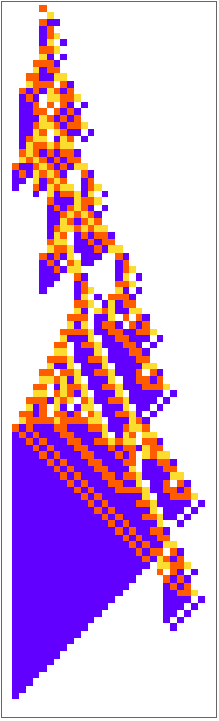
The application of its rule cases we think of as the “phenotype”. Starting from the same initial condition, the rule produces a reproducible sequence of cellular states and eventually reaches the terminal all-zero state:
Out[]=
How we create similar but not identical CAs?
How we create similar but not identical CAs?
For a true clinical trial though, the population needs to be unique. We can’t just make 400 copies of the same CA as that would lead to same genome, same behavior, same lifespan, same response to disease and treatment. Our base CA was made up of 4 unique colors or cell states, and to generate unique CAs here, we have the option of changing 3 cells each time. So each cell has the chance to be any of the 4 colors at one time, therefore the CA genome is 4 x 4 x 4 = 64 possible neighborhood configurations.
This is the genome of base CA (notice how each of the 64 cells have 1 of the 4 unique cell colors / states):
This is the genome of base CA (notice how each of the 64 cells have 1 of the 4 unique cell colors / states):
Out[]=

There are 64 unique rule positions, and we can replace each selected cell position with any of the other 3 cell states. This gives us 64 x 3 = 192 possible 1-bit mutations. But, we have to keep the white cell constant, so that leaves us with 63 mutable positions. Therefore the number of unique mutations possible by changing only 1-cell is 63 x 3 = 189.
Below we can see base CA genome fixed on top, and 5 mutated genomes below changing at just 1 cell color in each row:
Below we can see base CA genome fixed on top, and 5 mutated genomes below changing at just 1 cell color in each row:
Out[]=

Looking now at the pattern of one of these mutated “genomes” we can see how changing just one rule case can lead to large variation in the behavior of the resulting space-time pattern.
Here is an example of single-position mutation in the 64 cell genome of our base CA (arrow show color change from purple to orange):
Here is an example of single-position mutation in the 64 cell genome of our base CA (arrow show color change from purple to orange):
Out[]=

Here’s the new rule’s space-time pattern:
Out[]=
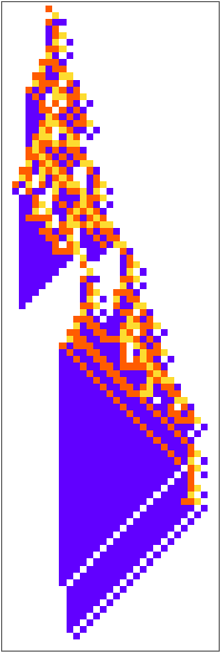
A single position mutation in the genome of a CA can lead to a variety of outcomes, each with varied boundary size, growth pattern, and lifespan length. This lays the foundation of selecting an appropriate population for our clinical trial.
Below we can see the base CA and five distinct single-bit mutated CAs:
Below we can see the base CA and five distinct single-bit mutated CAs:
Out[]=
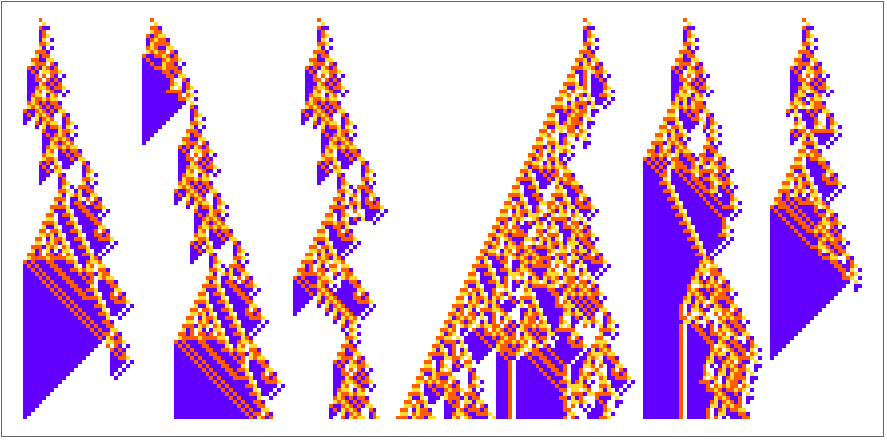
But “RandomRuleMutation” with single-bit mutations, only give us 189 unique combinations, so after a while, these patterns start repeating. And more importantly, 189 is not a big enough population to create a clinical trial dataset with.
2-bit Mutation CAs
2-bit Mutation CAs
With a 2-bit mutation, 2 cells in a genome are changed every time giving us a vast population size to choose our clinical trial dataset from.
◼
1 mutation : 63 x 3 / 1= 189
◼
2 mutation : (63 x 3 . 62 x 3) / 2 = 17,577
◼
3 mutation : (63 x 3 . 62 x 3 . 61 x 3) / 6 = 1,072,197
◼
4 mutation : (63 x 3 . 62 x 3 . 61 x 3 . 60 x 3) / 24 = 48,248,865
This is a crucial step for our population filters. Requesting more than 17,577 two-mutation draws cannot create more than 17,577 distinct two-mutation genotypes. Requesting RandomRuleMutation on a 50,000 or a 100,000 population will still give only 17,577 unique rules and most will be duplicates. Therefore, before even selecting our trial sample, we do de-duplicacy filters.
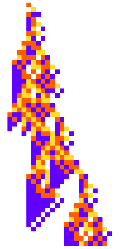
Below code shows the result of a CA with a 2-bit mutation (run the code below to visualize a different 2-bit mutation):
Out[]=
{{1,3,2},{6,0,2}} |

3-bit Mutation CAs
3-bit Mutation CAs
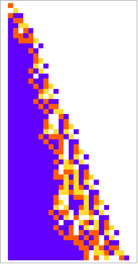
When we change 3 positions in the base CA genome, we get more than a million random mutated CAs. This also takes us further from the base CAs genetic makeup and introduces a true genetically diverse population to run a clinical trial on. Running a treatment on this population would check if a treatment is working on a diverse population and therefore confirm its efficiency. This is our way of making our CA clinical trial closer to human clinical trials.
In[]:=
mutated3 = RandomRuleMutation[ru, 3]Column [{ Select[Transpose[{Range[64],IntegerDigits[ru[[1]],4,64],IntegerDigits[mutated3[[1]],4,64]}],#[[2]]!=#[[3]]&],ArrayPlot[IntegerDigits[#[[1]], 4, 64] & /@ {ru, mutated3}, ColorRules -> colorrules, Mesh -> True, ImageSize->400],PlotCA[CellularAutomaton[mutated3, {{1}, 0}, {50, {-50, 50}}]] }]
Out[]=
{299459058088388517694360508545553198144,4,1}
Out[]=
{{20,1,2},{24,0,1},{35,1,3}} |

The need for so many CAs?
The need for so many CAs?
In human clinical trials, there is always a candidate pool from which a specific population are selected for final trial. Similarly, in our computational universe, “RandomRuleMutation” could generate a lot of duplicates, and we need to filter those out. Also, not every CA has the exact features or lifespan we are looking for. Thus, all these filters require us to have a large diverse population to choose from.
Increasing mutation level increased the number of distinct sampled rules, but it did not produce a monotonic increase in viable or unique CAs. The four-position dataset contained more distinct rules than the three-position dataset, but fewer survived the selected healthy-lifespan range. Greater access to rule space therefore generated both more diversity and more rules outside the trial’s viability definition.
Increasing mutation level increased the number of distinct sampled rules, but it did not produce a monotonic increase in viable or unique CAs. The four-position dataset contained more distinct rules than the three-position dataset, but fewer survived the selected healthy-lifespan range. Greater access to rule space therefore generated both more diversity and more rules outside the trial’s viability definition.
BUILDING A Clinical Trial ON CELLULAR AUTOMATA
BUILDING A Clinical Trial ON CELLULAR AUTOMATA
Trial Definitions:
Trial Definitions:
◼
BASELINE VIABLE : Baseline lifespan is strictly between 30 and 200.
◼
UNIQUE PHENOTYPE: Only one copy of each identical viable baseline trajectory is retained.
◼
TREATMENT APPLICABLE : After disease,the CA is still active at the planned treatment timestep and the treatment position lies within its active non-white spatial range.
◼
DISEASE ELIGIBLE : With Screen->True, the disease outcome is finite and shorter than that rule’s own healthy lifespan.
◼
TRIAL SELECTION POOL: The final dataset which can be chosen for Clinical Trial groups A and B.
◼
DESIRABLE OUTCOME: The final measured lifespan is within 80-120.
Preparing Trial Dataset
Preparing Trial Dataset
We prepare our trial dataset by first generating random rule mutations. Here we select 2-position mutations and a population diversity of 200,000. This gives us all the possible 2-position mutated CAs in a wide population, so even after removing duplicates we will have unique CAs to proceed with the trial.
◼
Function 1 : Generating mutation dataset
Once we have a diverse dataset, it is now time to filter based on lifespan range required for a trial. We do this to delete any extremely short-lived CAs with lifespan less than 15-20, and very broad range CA that go outside our study range above 200. For this we run a function that deletes duplicates and filters the entire CA population based on a range defined by the user. In our case, since our base CA has lifespan 101 steps, we set viable range {30, 200}. We filter the 200,000 mutated dataset generated in the previous step for CAs that fall only in our viable range and remove any duplicates, hence bringing the number down to 2152 which is our healthy unique population.
An important thing to note is that “unique” function removes phenotypic duplicates, which means no two CAs have the exact same cell trajectory. This prevents the final population from being filled with multiple individuals that are different genetically but behave identically in the experiment.
This is just population filtering, we have not added any disease or treatments yet.
◼
Function 2 : Preparing trial population
Function 2 generates a histogram that shows how the final healthy population is distributed across lifespans. This helps us see whether the population is concentrated around a narrow lifespan, broadly distributed, or biased toward the lower or upper filter boundary. The histogram therefore confirms not only how many individuals remain but also the baseline diversity of their healthy lifespans.
We now have a clinical trial population that -
1
.originated from the same base rule
2
.contains a chosen number of random rule mutations
3
.have healthy lifespans within the selected interval
4
.produce non-duplicate healthy trajectories
3. Defining Health, Disease, Treatment and Recovery
3. Defining Health, Disease, Treatment and Recovery
In cellular automata, a perturbation has a variety of effects on the same population. Therefore, it is crucial to label healthy, disease, and treated carefully.
Using the base CA as an idealized model of a “healthy organism” we can then frame disease as perturbations to the CA. Here we’re showing what happens when you change one cell in the pattern at different locations:
A CA can vary in lifespan length, boundary size, growth pattern, color states etc when perturbed. Moreover, a perturbation can act as a disease or a treatment for each CA. This co-relates with a drug showing different effects in different people. In our trial we focus on lifespan as a metric for defining disease and treatment. In the above example, we notice some perturbations shorten pattern length and lead to its early termination (all white state), while in other cases the pattern runs for a longer time or in some cases keeps growing outside of the base CAs healthy lifespan range (around 100 steps).
We can then model “treatment” as applying a subsequent perturbation to the CA in an “attempt” to bring it back to its original “healthy” state. Here we add different treatment perturbations to the base CA:
In the above example, we notice how 1 base CA reacts differently to the same treatment that is added at different time points. This proves that not just the perturbation, but its position coordinate is equally important for its effectiveness.
Therefore,in our exploration we’ll think of health as the length of the pattern i.e. the number of steps it takes until the pattern terminates in the all-white state. A “disease” is a perturbation that shortens lifespan of majority of CAs in a population.“Effectiveness” of the treatment will be defined as how closely it brings the CA back to its original lifetime of 101 steps. And “recovery point” will be a range close to healthy lifespan of our base CA (80-120).
Based on our exploratory analysis with a variety of perturbations at different time steps, cell states, and column widths’; we’ll see that treatment response depends on the computational genotype, the state reached after disease, the intervention and the endpoint used to judge recovery.
What qualifies as a disease?
What qualifies as a disease?
So far our trial population contains CAs that are already healthy, viable and non-duplicate. However, not every CA responds to the same perturbation in the same way. A perturbation may shorten one CAs lifespan, but have little effect on another. For this reason, we first apply the disease perturbation to the whole prepared population. We then keep only the CAs in which the disease produces a clear and finite harmful effect.
We use the function “makegroups” to apply the disease, screen the population and create the two trial groups. The disease screen filter keeps only CAs where AfterPLife < BaseLife. This means the disease must shorten the lifespan of that individual. The diseased lifespan must also be finite therefore preventing undefined or endless outcomes from entering the main screened trial.
Users have an option of switching this off if they do not want to use this filter by simply typing False here.
◼
Function 3: Disease screening and creating Control (A) and Treatment (B) groups:
Why Screen for Disease?
Why Screen for Disease?
The disease perturbation is the same for every CA, but the population is genetically diverse. Different genomes may respond differently.
A disease perturbation may:
- shorten lifespan
- make no difference
- increase lifespan
- create a non-finite outcome
Therefore, the perturbation should only be called a disease for the individuals where it actually causes measurable harm. This is similar to selecting patients who clearly show the disease condition before testing a treatment.
For our trial, the disease perturbation is: {16,203}->1
This perturbation is applied at timestep 16 and position 203. The cell state at that point is changed to state 1.
This perturbation is applied at timestep 16 and position 203. The cell state at that point is changed to state 1.
Eligibility Filters
Eligibility Filters
Disease eligibility and treatment eligibility are different checks. Disease eligibility asks whether the disease produces a finite lifespan shorter than that of the healthy base rule’s baseline. Treatment eligibility asks whether the planned treatment can actually be applied.
The treatment is fixed at timestep 24 and position 209. Mutated CAs can occupy different positions, and some diseased CAs may end before timestep 24. The “withinboundsQ” function builds the diseased CA and its active boundary. “withinboundsQ” then checks whether the treatment time still exists and whether position 209 lies inside the active, non-white part of that CA.
CAs that end before treatment, or have only white background at the treatment position, are removed before groups are made. The treatment is not applied during this check. It is only used to make sure every randomized CA could receive the same planned treatment.
Randomizing Trial Groups A and B
Randomizing Trial Groups A and B
After disease screening and treatment eligibility, the user can choose from the trial eligible pool an even number of patients to build the control and treatment arms of clinical trial. We then do a random sample pool to assign the CAs to equal groups. Randomization prevents us from intentionally choosing better CAs for the treatment group. It helps distribute different genomes and different baseline lifespans across both groups.
trial 1 = 2 bit mutation
Population diversity = 200,000
We had 2152 unique population, and after disease screening and treatment eligibility we filtered it down to 138.
From this 138, we choose 120 for our clinical trial.
trial 1 = 2 bit mutation
Population diversity = 200,000
We had 2152 unique population, and after disease screening and treatment eligibility we filtered it down to 138.
From this 138, we choose 120 for our clinical trial.
What qualifies as a Treatment?
What qualifies as a Treatment?
We ran “SeedRandom” testing on an independent diseased dataset to check the 10 top performing treatment perturbations that increase lifespan in majority population. For our trial, we selected {24, 209}-> 3 , as our treatment perturbation.
◼
Function 4: Adding treatment to group B and checking “AfterTreatmentLifespan”
Here the "Improved" field only means that treated lifetime exceeded diseased lifetime . It does not necessarily mean the CA reached the predefined desirable recovery range of 80–120.
◼
Function 5: Plotting healthy, disease, treated CAs for group B:
These results show that the same treatment does not affect every CA equally. Some CAs -
◼
improve
◼
show no change
◼
become worse
◼
improve far beyond their original healthy lifespan
◼
produce non-finite outcomes.
This variation is one of the main reasons for using a population-based clinical trial instead of studying only one CA.
This variation is one of the main reasons for using a population-based clinical trial instead of studying only one CA.
What qualifies as recovery?
What qualifies as recovery?
Improvement is not the same as recovery. A lifespan increase from 20 to 35 is an improvement, but it does not restore an organism to the reference lifecycle near 101. For this reason, the primary binary endpoint was defined as a final lifespan between 80 and 120. This range allows some natural variation around the reference lifespan.
The trial does not simply ask whether treatment increases lifespan. It asks whether treatment increases the number of CAs that return to a healthy-like lifespan range.
The trial does not simply ask whether treatment increases lifespan. It asks whether treatment increases the number of CAs that return to a healthy-like lifespan range.
The first complete validation trial used rules exactly two mutations away from the reference genome. This mutational distance provided a large search space while keeping the population connected to the reference organism.
6. RESULTS
6. RESULTS
1. Treatment response differed across mutation populations
1. Treatment response differed across mutation populations
The treated group had a higher desirable outcome rate in all three screened mutation populations. The observed difference was largest in the 2-bit trial and smallest in the 4-bit trial. This descending pattern describes the completed trials, but does not by itself prove that mutation level alone caused the reduction
2. Magnitude of treatment effect is highest in two-bit mutation population
2. Magnitude of treatment effect is highest in two-bit mutation population
Comparing percentage-point improvements makes the treatment effect directly comparable across trials despite different sample sizes.
The treatment benefit decreased from 15 percentage points in the two-mutation population to 8 percentage points in the three-mutation population and 4 percentage-points in the four-mutation population. The results therefore show a progressive reduction in observed treatment benefit across increasingly diverse populations.
The treatment benefit decreased from 15 percentage points in the two-mutation population to 8 percentage points in the three-mutation population and 4 percentage-points in the four-mutation population. The results therefore show a progressive reduction in observed treatment benefit across increasingly diverse populations.
3. Statistical significance is dependent on genetic diversity and sample size
3. Statistical significance is dependent on genetic diversity and sample size
The 2-bit and 3-bit screened trials were statistically significant. The 4-bit screened trial was not statistically significant, although the treated group still had more desirable outcomes. The absence of statistical significance therefore reflects greater uncertainty in the observed effect rather than evidence that the treatment produced no response.
4. Disease screening filter changed desirable outcomes and trial significance
4. Disease screening filter changed desirable outcomes and trial significance
With screening on, the control and treated desirable rates were 7.5 % and 15.5 %, producing an 8.0 percentage-point difference.
With screening off, the corresponding rates were 16.5 % and 19.5 %, producing a 3.0 percentage-point difference.
The screened comparison was statistically significant, whereas the un-screened comparison was not. This does not show that screening creates an effective treatment. It shows that eligibility criteria change the population and therefore change the question answered by the trial.
Result Summary : The grouped bar chart demonstrates that treatment consistently produced more desirable outcomes than disease alone. The second figure shows that this benefit became progressively smaller as mutation diversity increased. The Fisher exact analysis confirms that this reduction in effect was accompanied by decreasing statistical evidence.
7. Inference
7. Inference
What the experiments established
What the experiments established
1. A complete computational clinical trial pipeline was successfully implemented, including population generation, viability filtering, duplicate removal, perturbation-based disease modeling, optional eligibility screening, randomization, treatment application, missing outcome accounting, survival visualization, and exact statistical comparison.
2. The fixed treatment perturbation increased the observed number of desirable outcomes in all recorded trials, but the magnitude and certainty of this increase varied across populations.
3. The screened 2-bit and 3-bit trials showed significant differences, while the screened 4-bit trial did not. Therefore, the treatment cannot be described as universally effective across the tested rule populations.
4. The 3-bit screening comparison demonstrated that changing eligibility criteria can substantially change both the baseline outcome rate and the apparent treatment effect.
5. For the binary Fisher comparison, every randomized CA remained in the denominator. Any final lifetime outside (80–120) including an undetermined outcome, was counted as not desirable. Undetermined outcomes were reported separately.
8. What We Learned About Clinical Trials on Cellular Automata
8. What We Learned About Clinical Trials on Cellular Automata
◼
Disease and treatment are not intrinsic labels attached to perturbations . Their meanings emerge only after the perturbation interacted with a particular computational organism and a particular outcome definition.
◼
Longer lifespan is not automatically better. A treatment could lengthen life without restoring the reference range, or could create a non terminating trajectory. This led us to select a desired range for healthy-population definition.
◼
Eligibility criteria changes the trial outcome completely. Filters such as - finite-life, viable range {30-200}, uniqueness and disease-screening defined the population to which the treatment claim was applied.
◼
Early visible change was insufficient as a surrogate endpoint. The trial with timestep 30 as a metric was sensitive to disturbance but nearly uninformative about whether the final outcome would be shortening or extension of life.
The strongest overall thesis is therefore: treatment response is not an intrinsic property of an intervention alone. It is an emergent property of the interaction among intervention, organism, population definition, and endpoint.
9. Limitations
9. Limitations
◼
The project studies one abstract CA family and one main disease-treatment pair only.
◼
The 2-bit trial used 120 randomized CAs, while 3-bit and 4-bit used 400.
◼
Population generation was random simply based on genomic diversity of base rule.
◼
Phenotypic deduplication retains one genotype from potentially several rules producing the same healthy trajectory.
◼
Only one viability range, recovery range, and observation window were tested.
◼
Lifetime is an imperfect endpoint: non-termination can look undesirable in binary analysis but may be interpreted as survival in a time-to-event analysis.
10. Implications for Computational Biology, Medicine and Future WRI Research
10. Implications for Computational Biology, Medicine and Future WRI Research
This project produces a reusable experimental structure for running clinical trials on cellular automata.
The structure
The structure
A model supplies genomes, trajectories and perturbations. The trial layer supplies population generation, eligibility, randomization, endpoints, treatment discovery, independent validation and failure analysis.
Usability
Usability
1. This could influence future WRI medicine work by making population-level validation a standard part of perturbation experiments. Instead of displaying a few striking examples, a candidate disease or treatment could be evaluated across a declared population, with explicit exclusions and a specific validation protocol.
2. The framework also provides a synthetic controlled laboratory for precision medicine. Because every computational genotype and state is observable, future work can build maps from genotype and early phenotype to treatment response, identify responder subgroups and ask whether different treatments are optimal for different regions of rule space.
3. The lifespan as an endpoint is one of the many metrics that can show the success of a trial. We can explore boundary size, width of pattern, cell counts at a certain timestep etc.
4. The disease screening filter motivates a new experiment in which one criterion is removed at a time. This would determine whether non termination removal, the 30-200 range, phenotypic uniqueness and disease-shortening susceptibility each contribute independently to the stability of the treatment estimate.
Future directions
Future directions
The clinical trials on cellular automata offer a controlled setting in which the logical architecture of biological and medical reasoning can be made explicit, tested and improved before it is carried into more realistic models. We can plan to run trials with new treatment perturbations and even more diverse populations. Another direction would be to run this treatment on a new CA rule population.
Concluding Remarks
Concluding Remarks
This project developed a reusable computational framework for conducting population-based clinical trials on cellular automata. A fixed perturbational treatment produced considerable recovery toward a healthy-like lifespan in independently generated two- , three- and four - mutation populations, but not in a population lacking the same interpretive safeguards. Treatment was associated with a higher desirable-outcome rate in every screened population, but the magnitude of the difference declined from 15.0 to 8.0 to 4.0 percentage points. The two-position and three-position comparisons were statistically significant, while the four-position comparison was not. A separate three-position experiment showed that removing the disease-screening criterion reduced the treatment-control contrast and changed the statistical conclusion.The result supports cellular automata as heterogeneous virtual trial populations and identifies population definition as part of the treatment question itself.
Acknowledgments
Acknowledgments
I thank my mentors Willem Nielsen and David Debrota for their expertise and guidance that helped in the completion of this project. I am extremely grateful for their time and efforts. Additionally, I would like to thank Brian Mboya for Wolfram language coding help and assistance.
Most importantly, I sincerely thank Stephen Wolfram for suggesting a project topic that merged my biology expertise with Wolfram research in the best way possible. Overall, I thank all the mentors at WSRI, program director Stephanie Boyer and all the WSRI team for their efforts.
Most importantly, I sincerely thank Stephen Wolfram for suggesting a project topic that merged my biology expertise with Wolfram research in the best way possible. Overall, I thank all the mentors at WSRI, program director Stephanie Boyer and all the WSRI team for their efforts.
References
References
1
.S. Wolfram (2025), Towards a Computational Formalization for Foundations of Medicine, Stephen Wolfram Writings.
2
.S. Wolfram (2025), What’s Special About Life? Bulk Orchestration and the Rulial Ensemble in Biology and Beyond, Stephen Wolfram Writings.
3
.Wolfram Research (2026), CellularAutomaton, Wolfram Language Documentation.
4
.Wolfram Function Repository (2026), PerturbedCellularAutomaton, Wolfram Function Repository.
AI Disclosure
AI Disclosure
The following generative AI tools were used in this project: [OpenAI GPT 5.6Sol]. They were used for [ debugging code, testing alternative code logic, researching clinical trials literature]. All code and written content was reviewed, understood and approved by the author.
CITE THIS NOTEBOOK
CITE THIS NOTEBOOK
Running Computational Clinical Trials on Cellular Automata
by Iqra Sajid
Wolfram Community, STAFF PICKS, July 16, 2026
https://community.wolfram.com/groups/-/m/t/3762735
by Iqra Sajid
Wolfram Community, STAFF PICKS, July 16, 2026
https://community.wolfram.com/groups/-/m/t/3762735