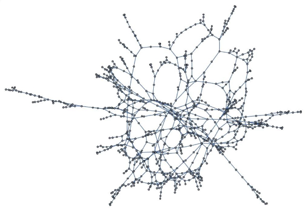
Hard spheres have been widely used in condensed matter as models for a variety of systems, such as liquids, crystals and glasses. While there exists extensive theoretical insight, as well as numerical data, much work is required for characterizing dense amorphous packings (glassy states). In this project we build upon current efforts to compute the observables of these systems by means of token-event graphs that summarize their dynamical evolution. We investigate the structure of these causal graphs and explore the possibility of drawing a parallel with the Feynman diagram construction to better understand the physical properties reflected in them.
Introduction
Introduction
About Hard Spheres
About Hard Spheres
Hard spheres are impenetrable particles of radius σ described by the pairwise potential
V(, ) =
r
1
r
2
|
(
1
)Systems composed of hard spheres can be studied by analytical means or by simulating the dynamical evolution, which is determined by pairwise perfectly elastic collisions between the particles.
Graphs in Traditional Physics
Graphs in Traditional Physics
Cluster theory
Cluster theory
Many statistical mechanical systems have an intricate connection with graph theory provided by Cluster expansion methods. These allow to compute configuration functions (e.g. correlation functions and free energies) of a variety of fluids in equilibrium. The idea, first implemented by Mayer and Montroll (1941), is that the thermodynamic functions can be expanded in a power series of density. An important example is the virial expansion for the pressure in low density nonpolar fluids:
P/(ρkT) = 1 + B(T)ρ + C(T) + ...
2
ρ
(
2
)where is Boltzmann’s constant and ,etc. are the virial coefficients. These coefficients can be calculated as cluster integrals involving possible combinations of pairwise interactions to the correspondent power in the expansion (2), which are in correspondence with all graphs with given topologies (Andersen, 1977).
k
B,C
This can be understood as a departure from the ideal gas behavior, with each correction involving an increasing number of particle interactions. If rather than thinking about the static configurations we consider the dynamical evolution, the claim is that the probability of a given pair of particles meeting again at different times implies a modification of the ideal gas statistics.
Feynman Diagrams
Feynman Diagrams
Another example of diagrammatic expansion in physics are Feynman diagrams, which are pictorial representations of the fundamental interactions in nature and the processes they describe. The idea behind them is that all processes can happen in an infinity of ways, each of them contributing to the total probability. Mathematically, this corresponds to computing the probabilities as a series of Feynman diagrams with all the possible graph topologies, which is called the Dyson-Wick expansion.
In practice, Feynman diagrams can be used to compute scattering amplitudes and correlation functions, examples from which are shown respectively in the pictures below (Peskin and Schroeder, 1995). The first one refers to the probability that some initial states with a given momenta evolve into a final states with other momenta by means of interactions. The later is a measure of the probability that two (or more) particles occupy positions and in spacetime, which indicates the structure of a many particle system.
x
y
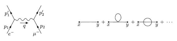
The structure of these diagrams is as follows. Loosely speaking, each line represents a particle and each vertex represents an interaction with a strength given by a coupling constant. For instance, in the picture above (left), two electrons interact by interchanging a photon and the strength of the interaction is the electron’s charge.
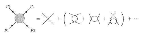
The easiest example for a theory containing only one species of particles is the - scalar theory, for which the scattering between two particles would look something like this (Peskin and Schroeder, 1995):
4
ϕ
Main Results
Main Results
1. Repository function for hard spheres
1. Repository function for hard spheres
The dynamical evolution of a hard sphere system can be implemented in Mathematica by means of the function HardSphereSimulation, which is a result of a previous Summer School project (Kafker, 2020). The basic functionality is as follows:
In[]:=
{simulation,graph,collisions,positions}=ResourceFunction["HardSphereSimulation"][Association[{"Positions"->Catenate@Table[{-10+2.5i,10-2.5j},{i,4},{j,4}],"Velocities"->Table[.5{1,-1},16],"BoundaryCondition"->"Reflecting","BoxSize"->20,"StepSize"->0.1,"ParticleRadius"->1,"Steps"500,"Output"->{"Visualize","CausalGraph","Collisions","PositionsByTime"}}]];
In[]:=
graph=graph//setLabels["Automatic"];Row[{simulation,graph}]
Out[]=


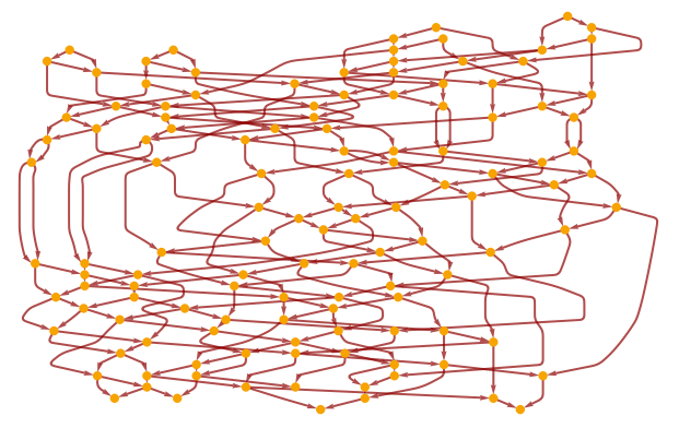
The “Output” option allows us to get all the relevant phase space information, such as the positions and velocities at each step of time. Additionally, the function can return a causal graph in which each vertex is a collision of the form {, , time} (shown here as s). Accordingly, each edge represents a particle in the initial or final state of the collision. The function setLabels allows to set the to show the collision or its index in the , it can be found in an initialization cell at the end of the notebook.
particle
i
particle
j
2. CausalGraphs in spacetime
2. CausalGraphs in spacetime
While the causal graph reflects the causal relation between collisions, it doesn’t keep track of the positions at which they occur. This is not a problem in the present case because the system is classical, but it could be troublesome in a relativistic situation in which the time ceases to be absolute. If one is interested in looking at the whole picture, a possibility is to draw the worldlines of the particles. For that, we set the vertex coordinates to the positions of the collisions in spacetime (which can be done only for 1+1 and 2+1 dimensions):
In[]:=
spaceTimeGraph::nnarg="The dimension `1` of collisions is not 1 or 2";spaceTimeGraph[graph_,positions_,size_:Small]:=Module[{dim,collisions,timePartColl,posColl,vertexCoord},dim=Length@positions[[1,1]];collisions=VertexList@graph;timePartColl=Reverse/@collisions[[All,{1,3}]]/.{a_,b_}->{IntegerPart[10a],b};posColl=positions[[Sequence@@#]]&/@timePartColl;vertexCoord=MapThread[Append,{posColl,collisions[[All,3]]}];Switch[dim,1,Graph[graph,VertexCoordinates->Thread[collisions->vertexCoord],AxesTrue,ImageSizeSmall],2,Graph3D[graph,VertexCoordinates->Thread[collisions->vertexCoord],AxesTrue,AxesLabel->{"x","y","t"},LabelStyle15,AspectRatio{1,1,2},ImageSizesize,PlotTheme"Minimal"],_,Message[spaceTimeGraph::nnarg,dim]]]
In[]:=
spaceTimeGraph[graph,positions]
Out[]=

3. Following particles in the CausalGraph
3. Following particles in the CausalGraph
Given the importance of re-collisions between particles, it is interesting to highlight the paths of individual particles in the causal graph and see how many times they meet each other during the simulation. We can do that with the following functions.
First, we construct a path along the graph by going through the vertices, following at each step the edge that corresponds to the initial particle (the function can be easily generalized to other criteria to decide which edges to follow).
Then we can highlight the paths the two particles that participate in the collision with index startIndex:
For the same graph from the previous section:
If one neglects the rest of the particles, this looks like a two-point diagram with loops.
4. Another kind of graph
4. Another kind of graph
Here we implement a new graph that can reflect the dynamical evolution of the system. The idea is to invert the roles in the causal graph: the vertices are now the particles. Two vertices will be adjoint if the particles have collided during the simulation, and the adjacency weight is given by the number of collisions between them:
For a new simulation in 3D:
It is interesting to look at the evolution of this graph during the simulation. For that we implement the following function:
Concluding Remarks
Concluding Remarks
In this project we were able to visualize the causal relations between the collisions in a hard sphere simulation in different ways. We found some hints of similarity with cluster and Feynman diagrams, but we were not able to establish a suggestive connection. In order to achieve this, one possibility would be to explore the evolution of the same system many times and analyze how the possible topologies of the causal graph are related to the statistics of re-collisions between particles.
Acknowledgments
Acknowledgments
I would like to thank my mentors: Alejandra Ortiz, for her incredible patience and determination to overcome the initial difficulties; and Paul Abbott, for giving me useful material and coding advice during the whole school. I am also grateful to Xerxes Arsiwalla and Hatem Elshatlawy for useful discussions. Special thanks to Stephen Wolfram for providing the idea for this project, and to the rest of the staff for making this school such an amazing experience. I had the pleasure of meeting incredible people and learning so many new things that I am sure will shape my way forward.
References
References
1
.Peskin, M. E. and Schroeder, D. V. (1995), An Introduction to Quantum Field Theory. Taylor & Francis Group LLC.
2
.Parisi, G. and Zamponi, F. (2010). “Mean-field theory of hard sphere glasses and jamming”. Rev. Mod. Phys. 82, 789. https://doi.org/10.1103/RevModPhys.82.789
3
.Mayer, J. E. and Montroll, E. (1941), “Molecular distributions”, J. Chem. Phys. https://doi.org/10.1063/1.1750822
4
.Andersen, H.C. (1977). Cluster Methods in Equilibrium Statistical Mechanics of Fluids. In: Berne, B.J. (eds) Statistical Mechanics. Modern Theoretical Chemistry, vol 5. Springer, Boston, MA. https://doi.org/10.1007/978-1-4684-2553-6_1
5
.Kafker, M. (2020). “Exploring Networks in Hard Sphere Models”. Retrieved from: https://community.wolfram.com/groups/-/m/t/2028871
Cite This Notebook
Cite This Notebook