This project demonstrates how to use Wolfram Language’s built-in neural network framework to automatically detect cracks in concrete surface images. The model follows Gabriel Atkin’s neural network and is trained on the widely used Kaggle Concrete Surface Crack Detection dataset, which contains 40,000 labeled RGB images of concrete surfaces, evenly divided between crack-free (negative) and cracked (positive) samples.
In[]:=
$HistoryLength=0;
In[]:=
mydir=SetDirectory[NotebookDirectory[]];
The dataset was generated from 458 high-resolution photographs of concrete structures and includes a wide variety of surface textures and lighting conditions. Each image has a resolution of 227 × 227 pixels and is labeled for binary image classification. No artificial data augmentation such as rotation, flipping, or tilting was applied during dataset creation, making it a realistic benchmark for crack detection.
Because we are working with a large volume of images, it is more efficient to download the dataset directly and use the uncompressed files locally rather than relying on the built-in Kaggle link.
file=URLDownload["https://www.kaggle.com/api/v1/datasets/download/arunrk7/surface-crack-detection",FileNameJoin[{mydir,"surface-crack-detection.zip"}]];
In[]:=
ExtractArchive[file];
There are 20,000 files in each category:
In[]:=
{pos,neg}=FileNames[FileNameJoin[{mydir,#,"*"}]]&/@{"Positive","Negative"};
In[]:=
Length/@{pos,neg}
Out[]=
{20000,20000}
Select a subset of the indices and partition it into training, validation, and test sets with sizes {3800, 400, 15000}, corresponding to 3,800 training samples, 400 validation samples, and 15,000 test samples, respectively.
In[]:=
split={3800,400,15000};pool=Range[20000];
In[]:=
TraingValidationTestSets[data_,size_List]:=BlockMap[Complement@@#&,FoldList[Complement[#1,RandomSample[#1,#2]]&,pool,size],2,1]
In[]:=
tvtPos=TraingValidationTestSets[pos,split];tvtNeg=TraingValidationTestSets[neg,split];
Efficient Loading of Large Image Datasets:
In[]:=
LaunchKernels[];
In[]:=
allNegImg=Flatten@ParallelMap,neg;allPosImg=Flatten@ParallelMap,pos;
◼
Sample crack-free (Negative) images
In[]:=
Grid[Partition[RandomSample[allNegImg,6],3]]//Framed
Out[]=
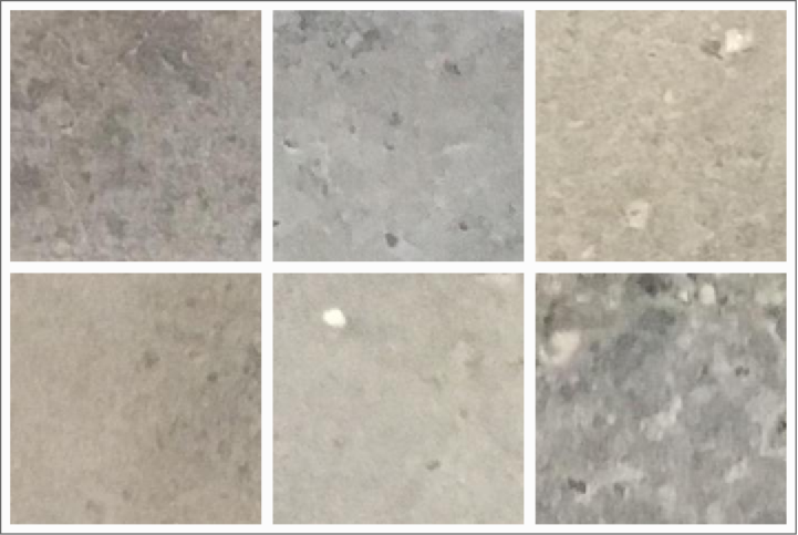
◼
Sample images with cracks (Positive)
In[]:=
Grid[Partition[RandomSample[allPosImg,6],3]]//Framed
Out[]=
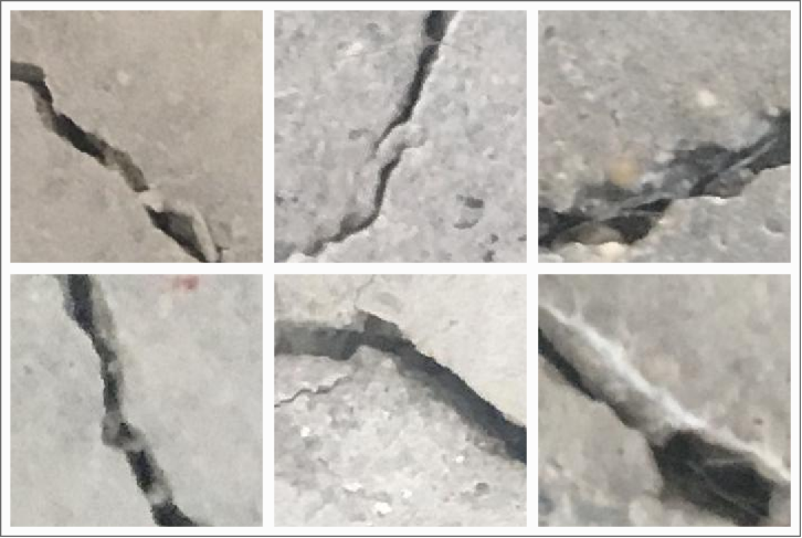
Convert the index set into the corresponding labeled images and shuffle within the sets:
In[]:=
{tr,vld,tst}=Table[RandomSample[Join[#->{0}&/@(allNegImg[[tvtNeg[[k]]]]),#->{1}&/@(allPosImg[[tvtPos[[k]]]])],2*split[[k]]],{k,3}];
Follow Gabriel’s source code to create a simple neural network for image classification and initialize it:
In[]:=
net=NetChain[{ConvolutionLayer[16,{3,3}],ElementwiseLayer[Ramp],PoolingLayer[{2,2},{2,2}],ConvolutionLayer[32,{3,3}],ElementwiseLayer[Ramp],PoolingLayer[{2,2},{2,2}],AggregationLayer[Mean],LinearLayer[1],LogisticSigmoid},"Input"->NetEncoder[{"Image",{120,120},ColorSpace->"RGB"}]];net=NetInitialize[net]
Out[]=
NetChain


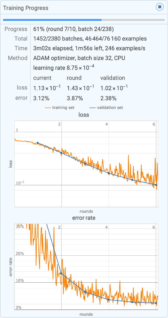
Train the network using the training and validation datasets. Although GPU acceleration is recommended, the dataset remains small enough to be trained on a CPU. In benchmark tests, a laptop NVIDIA Quadro P2000 achieved training speeds approximately 6–8 times faster than an Apple M1 Max for this task.
In[]:=
trained=NetTrain[net,tr,LossFunction->CrossEntropyLossLayer["Binary"],BatchSize->32,ValidationSet->vld]
Out[]=
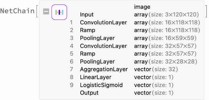
Check basic information for the trained net:
In[]:=
Information[trained]
Out[]=
Check the accuracy of the trained neural network on test data:
In[]:=
NetMeasurements[trained,tst,"Accuracy"]
Out[]=
0.9747
Visualize the confusion matrix:
In[]:=
NetMeasurements[trained,tst,"ConfusionMatrixPlot"]
Out[]=
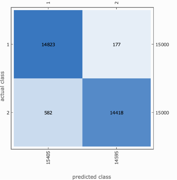
Here, Class 1 corresponds to the Negative class (no crack present), while Class 2 corresponds to the Positive class (crack present).
This can be verified by applying the trained network to the positive images in the test set and examining the resulting predictions.
Compare to the numeric values from the confusion matrix:
Visualize the Receiver Operating Characteristic (ROC) curve for the trained model. The curve lies very close to the upper-left corner of the plot, indicating a high true positive rate and a low false positive rate. This suggests that the network performs very well at distinguishing between cracked and non-cracked concrete surfaces:
Create a simple application to classify images of concrete surfaces.
A blue dot above an image indicates that the network’s prediction is correct, while a red dot indicates an incorrect prediction:
A blue dot above an image indicates that the network’s prediction is correct, while a red dot indicates an incorrect prediction:
Summary
Summary
Using Wolfram’s neural network functions, the project covers data loading, preprocessing, training, validation, and model evaluation. The resulting classifier can accurately distinguish between healthy concrete surfaces and surfaces containing cracks, demonstrating how machine learning and image processing can assist civil engineers in structural inspection and condition assessment. Such automated inspection tools can help improve the speed, consistency, and reliability of building health monitoring.
CITE THIS NOTEBOOK
CITE THIS NOTEBOOK
Concrete crack classification with deep learning
by Shenghui Yang
Wolfram Community, STAFF PICKS, June 6, 2026
https://community.wolfram.com/groups/-/m/t/3728193
by Shenghui Yang
Wolfram Community, STAFF PICKS, June 6, 2026
https://community.wolfram.com/groups/-/m/t/3728193