Transient Heat Conduction Using Chebyshev Collocation
Authors: Housam Binous and Ahmed Bellagi
Transient Heat Conduction Using Chebyshev Collocation
Authors: Housam Binous and Ahmed Bellagi
Authors: Housam Binous and Ahmed Bellagi
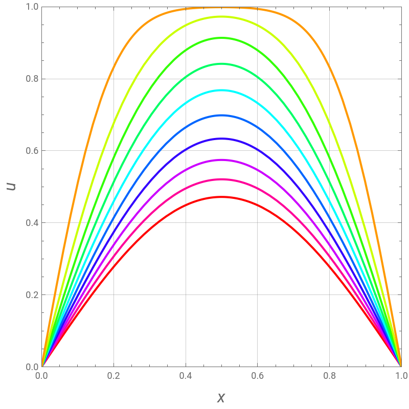
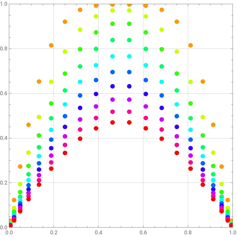
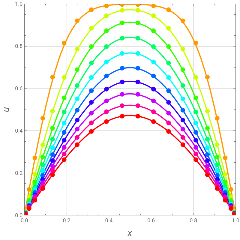
In the discrete Chebyshev–Gauss–Lobatto case, the interior points are given by =cos(jπ/N). These points are the extrema of the Chebyshev polynomial of the first kind (x).The Chebyshev derivative matrix at the quadrature points, , is an matrix given by=, =-, = for , and =(-1)(-) for and ,where =1 for and ==2.The second-order partial spacial derivatives are obtained using =.An affine transformation, , allows shifting from interval to.Detailed information on the Chebyshev orthogonal collocation as well as its application in the CHE curriculum are available in Refs. 1-5.Consider the one-dimensional heat equation given by=u, with and .This equation represents heat conduction in a rod. The boundary conditions are such that the temperature, , is equal to 0 at both ends of the rod: and for . Without loss of generality, one can take the thermal diffusivity, , equal to . The initial condition is given by for The temperature can be found using either NDSolve (solid colored curve) or the Chebyshev collocation technique (colored dots). Both methods give the same results, which are plotted in the same diagram at various values of time, ranging from 0.01 to 0.1 with a span of 0.01. You can change the number of interior points used by the Chebyshev collocation method. Finally, the results using Python are compared to the solution using Mathematica.References:[1] L. N. Trefethen, Spectral Methods in MATLAB, Philadelphia: SIAM, 2000.[2] H. Binous, A.A. Shaikh and A. Bellagi, (2015), Chebyshev orthogonal collocation technique to solve transport phenomena problems with Matlab® and Mathematica. Comput Appl Eng Educ, 23: 422-431. https://doi.org/10.1002/cae.21612[3] H. Binous, S. Kaddeche and A. Bellagi, Solving two-dimensional chemical engineering problems using the chebyshev orthogonal collocation technique, Computer Applications in Engineering Education, 24(1), pp. 144-155, 2016. https://onlinelibrary.wiley.com/doi/abs/10.1002/cae.21680[4] H. Binous, S. Kaddeche, A. Abdennadher and A. Bellagi, (2016), Numerical elucidation of three-dimensional problems in the chemical engineering graduate curriculum. Comput Appl Eng Educ, 24: 866-875. https://doi.org/10.1002/cae.21756[5] H. Binous, S. Kaddeche and A. Bellagi, Solution of six chemical engineering problems using the Chebyshev orthogonal collocation technique. Comput Appl Eng Educ. 2017; 25: 594–607. https://doi.org/10.1002/cae.21823
y
j
T
N
(N+1)×(N+1)
D=
d
jk
0≤j,k⩽N
(N+1)×(N+1)
d
00
2+1
2
N
6
d
NN
2+1
2
N
6
d
jj
-
y
j
21-
2
y
j
1≤j≤(N-1)
d
jk
j+k
c
j
c
k
y
j
y
k
0≤j,k⩽N
j≠k
c
j
1≤j≤N-1
c
0
c
N
D
2
2
D
x=(y+1)/2
[-1,1]
[0,1]
1
α
∂u
∂t
2
∂
∂
2
x
t≥0
0≤x≤1
u
u(x=0,t)=0
u(x=1,t)=0
t≥0
α
1/s
2
cm
u(x,0)=1
0≤x≤1.
t
In[]:=
sol=NDSolve[{D[u[x,t],{t,1}]D[u[x,t],{x,2}],u[1,t]0,u[0,t]0,u[x,0]1-1Exp[-1000x^2(1-x)^2]},u,{x,0,1},{t,0,10}];plt1[i_]:=Plot[u[x,t]/.sol/.ti,{x,0,1},FrameTrue,GridLinesAutomatic,PlotStyle{Thick,Hue[i10]},ImageSize400{1,1},PlotRange{{0,1},{0,1}},PlotLegendsSwatchLegend[{Hue[i10]},{i},If[i0.1,LegendLabel"time",LegendLayoutAutomatic]],AspectRatio1,FrameLabel{Style["x",Italic,16],Style["u",Italic,16]}];p1=Show[plt1[0.1],plt1[0.09],plt1[0.08],plt1[0.07],plt1[0.06],plt1[0.05],plt1[0.04],plt1[0.03],plt1[0.02],plt1[0.01],PlotRange{{0,1},{0,1}}]
Out[]=


In[]:=
Npp=20;(*numberofinteriorpoints*)Np=Npp+1;(*constructingthedifferentiationmatrix*)d[0,0]=(2Np^2+1)/6//N;d[Np,Np]=-(2Np^2+1)/6//N;y[i_]:=Cos[iPi/Np]//N;d[i_,i_]:=-y[i]/(2(1-y[i]^2))//N;d[j_,k_]:=If[j≠k&&k≠0&&k≠Np&&j≠0&&j≠Np,(-1)^(j+k)/(y[j]-y[k])]//N;d[Np,0]=-1/2(-1)^Np;d[0,Np]=1/2(-1)^Np;d[j_,0]:=If[j≠Np&&j≠0,-1/2(-1)^j/(1-y[j])];d[j_,Np]:=If[j≠Np&&j≠0,1/2(-1)^(j+Np)/(1+y[j])];d[0,j_]:=If[j≠Np&&j≠0,2(-1)^j/(1-y[j])];d[Np,j_]:=If[j≠Np&&j≠0,-2(-1)^(j+Np)/(1+y[j])];Add=Table[d[i,j]//N,{i,0,Np},{j,0,Np}];Bdd=Add.Add;
In[]:=
upp[i_][t_]:=4Bdd[[i,j]]u[j][t];(*thesecondorderpartialderivativewithrespecttox*)
Np+1
∑
j=1
Eq[i_]:=u[i]'[t]upp[i][t];(*definingthesystemofODEsandtheinitialconditions*)sys1=Table[Eq[i],{i,2,Np}];BC1=u[1]'[t]0;BC2=u[Np+1]'[t]0;sys=Join[{BC1,BC2},sys1];init=Table[u[i][0]If[i1||iNp+1,0,1],{i,1,Np+1}];
sol2=NDSolve[Join[sys,init],Table[u[i][t],{i,1,Np+1}],{t,0,10}];(*solutionoftheabovesystemsofODEsbyNDSolve*)
In[]:=
plt2[j_]:=ListPlot[{Table[{1/2(y[i-1]+1),u[i][t]/.sol2/.tj//First},{i,Np+1,1,-1}]},PlotMarkersStyle["●",12,Hue[10j]],FrameTrue,GridLinesAutomatic,PlotRange{{0,1},{0,1}},ImageSize400{1,1},AspectRatio1];
In[]:=
p2=Show[Table[plt2[i],{i,0.01,0.1,0.01}],PlotRange{{0,1},{0,1}}](*plottingthesolution*)
Out[]=
In[]:=
Show[p1,p2](*comparisonofsolutionsobtaineddirectlywithNDSolveanditscounterpartusingChebyshevorthogonalcollocation*)
Out[]=
comparing the solutions obtained with Mathematica and Python