Traditionally, the stag hunt is a game theory situation in which hunters are given the choice between the better communal outcome, or guaranteeing a smaller reward for themselves. Either the hunter can go after the stag, which yields the player a bigger reward, or defect to hunt a hare, which will guarantee a smaller one. The game has two Nash equilibria, one in which everyone cooperates on the stag and one in which everyone defects to the hare. The stag is the payoff-dominant strategy because it produces the highest reward when everyone cooperates, while the hare is the risk-dominant strategy because it guarantees a reward even when the other players defect. Whether a group reaches the payoff-dominant equilibrium depends on whether each hunter is assured the others will reciprocate, and no hunter observes the whole group. In this essay, I model the hunters as agents on a random graph, where each agent updates its choice using only what its neighbors chose, in order to test which network conditions carry a group to the payoff-dominant equilibrium.
Introduction
Introduction
Which conditions allow groups to reach the higher valued but riskier consensus, and what causes a group to get stuck on the lower valued safer option? This is the assurance dilemma: each player fears their effort will be wasted if the others do not reciprocate, so they take the action that is guaranteed to benefit them individually rather than risking the collective one. The result is that a group can settle on the hare even when every member would prefer the stag, and once it does, no individual has a reason to break away alone.
I decided to model this by updating the probability of an agent picking a particular option based on which state produced the highest value, looking only at its neighbors. The agents sit on the vertices of a random graph, so each one observes only the agents it is connected to. I loop this until all the agents reach consensus, and then I run it across fifty graphs at once so I can see how changing one parameter affects the probability of landing on Stag or Hare. My graph shows the states the agents pick updating as it loops through.
Calculating Math for the Stag Hunt
Calculating Math for the Stag Hunt
This is the payoff table for a simple Stag Hunt.
Stag | Hare | |
Stag | {2,2} | {0,1} |
Hare | {1,0} | {1,1} |
This matrix shows the outcome based on what the hunters chose. They both get the higher valued reward if they both choose the Stag, while if they choose the Hare they get the guaranteed smaller reward without the risk of coming away with nothing.
We can calculate the probability of opponents cooperation using the Mixed-Strategy Nash Equilibrium:
The probability =)
This equals:
The probability =
(d-c)/((a-b)+(d-c)
This equals:
1/2
We can then plug that value into the Expected Value formula which is:
- P = Probability of the outcome
- O = The value of that outcome
- P = Probability of the outcome
- O = The value of that outcome
EV(P1*O1)+(P2*O1)+...+(Pn*On)
The Expected Value of both the Stag and the Hare are 1. That means that neither in this scenario is better.
However my matrix looks more like this:
Out[]=
Stag | Hare | |
Stag | {4,4} | {0,3} |
Hare | {3,0} | {3,3} |
In this scenario the Hare would be statistically better. The Expected value of hunting a Stag in this scenario is 1 while the Expected Value for hunting a Hare is 3.75.
In my model, the agents will be blind to the expected values. They will start out with an equal chance of choosing one of the states. All learnings will be based on observing which choice yielded the better outcome.
Creating the Basic Payoff Function
Creating the Basic Payoff Function
I began by making a function to represent the scores for the chosen states. I set a threshold, which is the percentage of their neighbor hunters that must choose stag for the value of the stag to be worth 4 instead of 0. The threshold will be 0.5 because it will be the simplest to keep as the baseline.
This function takes arguments in the form of the agent’s value S or H, and a corresponding list of all their neighbor’s choices:
In[]:=
c=.5;value[a_,b_]:=Which[MatchQ[a,"H"],3,MatchQ[a,"S"]&&Count[b,"S"]/Length[b]>c,4,MatchQ[a,"S"]&&Count[b,"S"]/Length[b]<=c,0];
I initialize my function so I can use it later:
value["S",{"H","S","S","S"}]
Out[]=
4
Creating the Network of Agents
Creating the Network of Agents
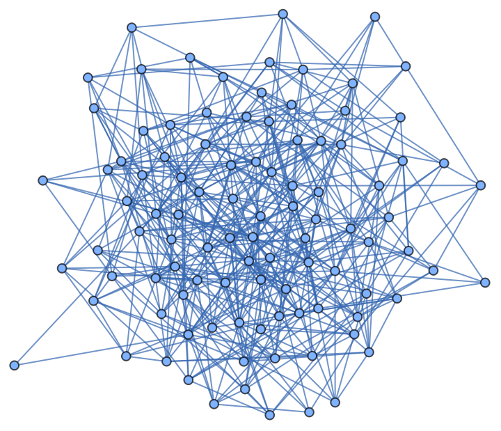
In this part I will construct the network of agents. I will generate a random graph to set up the agents and who their neighbors are. This code will pull out the agents themselves and which other agents are their neighbors. Here, I also set the initial probability values of choosing either Stag or Hare.
This part takes how many agents (vertices) and how many total connections (edges) I want and extracts the list of the agents themselves and their neighbors:
In[]:=
ClearAll[chooseGraph]chooseGraph[{n_Integer,m_Integer}/;m>=2*n]:=(g=RandomGraph[{n,m}];g=VertexDelete[g,Pick[VertexList[g],VertexDegree[g],0]];g=IndexGraph[g];vertices=VertexList[g];neighbors=AdjacencyList[g];g)chooseGraph[{100,450}]
Out[]=
Below I set the original values equal to a 50% chance of choosing Stag (ps) and a 50% chance of choosing Hare (ph):
In[]:=
n=Length[vertices];ps=.5;ph=.5;newPValues=Table[{ps,ph},n];
Defining the Agents’ States and Calculating the Values
Defining the Agents’ States and Calculating the Values
The main idea is that agents learn each round based on which state they see performs the best. This then updates their “opinion” on which choice is better. This opinion is represented by the probability score. Each time the following three functions are run, the probability scores will be updated. This function is responsible for taking two probabilities, turning them into the states, and finding the new list of values.
This function uses the assigned probability values to pick either Stag or Hare and outputs a list of all the agents’ values:
In[]:=
state[input_]:=(probAssoc=Association[Thread[VertexList[g]->Table[input[[i]],{i,n}]]];probAssocValues=Values[probAssoc];chosenstates=Map[RandomChoice,Table[input[[i]]->{"S","H"},{i,n}]];stateAssoc=Association[Thread[VertexList[g]->chosenstates]];valuesvertices=Values[stateAssoc];neighborvalues=Map[Replace[stateAssoc],neighbors,2];vertexlist=Partition[Riffle[valuesvertices,neighborvalues],2];values=value@@@vertexlist;values)
This initializes the payoff function:
In[]:=
state[newPValues]
Out[]=
{3,0,3,4,0,4,3,4,4,3,0,0,4,3,3,3,3,0,3,4,4,3,0,0,3,0,3,0,3,3,0,3,0,0,0,0,3,3,4,0,0,0,3,4,3,0,3,3,4,3,3,4,4,4,3,3,3,4,4,4,0,3,0,3,0,3,3,4,3,3,3,0,4,3,0,3,3,3,0,0,3,4,0,3,3,3,0,0,3,3,4,3,0,0,0,3,0,0,3,3}
Processing the Values so that the New Weights Can be Calculated Based on Neighbor Performance
Processing the Values so that the New Weights Can be Calculated Based on Neighbor Performance
Those values are then processed so that the agents are able to view both their neighbors’ and their own scores. Because we know what state each value maps to, we do not have to worry about what the state is here because all 4s and 0s will represent Stag, and all 3s will represent Hare. The point is that each agent will be influenced, and increase their probability of choosing a certain value, based on how many of their neighbors chose the right value. To make just the winner influence the agents’ new probability, I can simply set 3 equal to 0 if there exists a four, since the four would be the winning value, or leave the list be.
This function takes values and calculates how many of the winning values the agent will be influenced by and threads it with the current probability values:
In[]:=
ClearAll[extractingValues]findnowValues[now4_,now3_]:=Which[now4>0,{now4,0},True,{0,now3}];extractingValues[values_]:=(listOfNeighborChoices=Table[Table[values[[neighbors[[j]][[i]]]],{i,Length[neighbors[[j]]]}],{j,Length[neighbors]}];listOfChoices=MapThread[Prepend[#1,#2]&,{listOfNeighborChoices,values}];listOfAnswers4=MapThread[Count[#1,4]&,{listOfChoices}];listOfAnswers3=MapThread[Count[#1,3]&,{listOfChoices}];listOfAnswerLists=Partition[Flatten[Riffle[listOfAnswers4,listOfAnswers3]],2];listOfnowValues=findnowValues@@@listOfAnswerLists;probwithvalues=Partition[Riffle[listOfnowValues,probAssocValues],2])
This initializes the value-extraction function:
In[]:=
extractingValues[values];
Calculating the New Probability Weights
Calculating the New Probability Weights
The new probability values are computed by taking the original values and multiplying them by a learning factor, I chose 1.1 to hopefully see how the network updated, and raised that to the number of agents that chose the right state. Note that for the losing state, it is raised to 0 so there will be no change. This is then scaled down so that the new weights can be fed back into the loop to recalculate the state and so on to get a new probability.
This function multiplies the original probability by a factor raised to the number of winning conditions before scaling down the values to a sum of 1:
newValues[{{now4_,now3_},{ps_,ph_}}]:=Module[{ss,sh,nph,nps},ss=ps*(1.1)^now4;sh=ph*(1.1)^now3;nps=ss/(ss+sh);nph=sh/(sh+ss);newprobAssocValues={nps,nph}]
Creating the Repeating Function and Looping Through Until Consensus
Creating the Repeating Function and Looping Through Until Consensus
The idea here is that the prior three functions, state[], extractingValues[], and newValues[], are to be repeated until group consensus is reached. Every time, they update the agents’ probability values to become more skewed to the “better” value. It also shows the states updating until it reaches consensus.
This function sets the colors based on whether the state is Stag or Hare:
In[]:=
valueToColorList[vals_]:=Table[If[vals[[i]]=="H",Directive[Red,EdgeForm[Red]],Directive[Green,EdgeForm[Green]]],{i,Length[VertexList[g]]}];valueToColorList[chosenstates];
This function takes the newPValues and calls the three functions that must be repeated:
In[]:=
repeatingFunction[input_]:=(Table[AnnotationValue[{g,i},VertexStyle]=valueToColorList[chosenstates][[i]],{i,Length[VertexList[g]]}];state[input];extractingValues[values];Pause[2];newPValues=Map[newValues,probwithvalues])
This loops the repeatingFunction until all the states are the same:
Sample Progression of States
Sample Progression of States
Here I show a sample of how the states progress until they reach consensus. We can see the graph starts out almost equally split between the states, and slowly becomes all green as the agents “learn” from one another.
Calculating 50 Networks at a Time
Calculating 50 Networks at a Time
In the previous sections I have a way to choose a graph and see it updating. In this part, I am able to compute 50 graphs at once to collect lots of data at the same time. I can change a parameter and figure out roughly the probability of it landing on stag or hare.
This sets all the lists to 0:
This generates the graphs:
This function runs all fifty graphs and records each consensus:
This runs the batch across all fifty graphs:
This shows how many graphs reached Stag and how many reached Hare:
Conclusion
Conclusion
My project has built a way to analyze what type of networks and conditions allow groups of agents to reach the better, riskier consensus instead of being stuck on the safer option. I began by running fifty graphs at a time, each holding 50 agents, with the edge counts sweeping from 150 to 250. Roughly 40 of the fifty reached consensus on Stag and roughly 10 reached consensus on Hare, and every graph reached one of the two equilibria. When I repeated the batch the ratio stayed close to the same. If the number of connections made no difference, the difference between reaching Stag consensus verses Hare consensus would be based on chance. That would mean that every time I run these calculations the ratios between the outcome would vary more. Instead the same proportion kept appearing, which led me to believe that the number of edges made a difference.
I then analyzed individual graphs across that range of edge counts and found that there was a rough ratio between the number of agents and the number of connections at which the outcome switches from consensus on Hare to consensus on Stag as the connections increase. This is not a hard threshold. Every graph is generated randomly, so two graphs holding the same number of edges are still different graphs, and near the transition either outcome is possible depending on which one is drawn. Well below it the network practically always settles on Hare and well above it the network settles on Stag, but in between the result depends on the particular graph. To check whether this was a property of the size of the network or of how connected it was, I repeated the experiment with 100 agents while holding the ratio of edges to agents in the same range, and the results were similar.
This suggests that what carries a group to the payoff-dominant equilibrium is not how many agents the group contains, but how densely how connected those agents are. The reason this matters is that assurance is usually treated as something that exists between players, a question of whether each one trusts the others to reciprocate. In this model it also has a structural component.
Future Directions
Future Directions
In these past weeks, I have built an engine to compute outcomes based on different input values. One of my main goals in the future is to explore what types of situations yield the optimal outcome and what the threshold is. The direction I most want to pursue is analyzing the structure of the network itself, rather than only the number of connections it contains. The graphs I used here are random graphs, in which every possible edge is equally likely. This means they have very little clustering and no agents that are far more connected than the rest, which is not how most real groups are organized.
To test this I would hold the number of agents and edges constant, and vary the type of network. In the real world people cooperate in many different kinds of scenarios. Some groups are fully connected, so that everyone can see everyone else. Others are centered on a few agents who hold most of the connections, while the rest hold very few. Comparing these networks against the random graphs I used here would show whether the consensus depends on how the edges are arranged and not only on how many there are.
If a particular structure reliably carries a network to the payoff-dominant equilibrium, then the stag hunt becomes a design question. Instead of asking whether a group will cooperate, I would be asking how a group should be connected so that it does, which is a way of manufacturing assurance without changing the payoffs or the agents themselves.
References
References
1. iMotions. (2024). The stag hunt (game theory). https://imotions.com/blog/learning/research-fundamentals/the-stag-hunt-game-theory/
2. Majumder, K. (2025). [WSRP25] Visualizing the problem of distributed consensus for environmental attitudes [Notebook]. Wolfram Community. https://community.wolfram.com/groups/-/m/t/3502732
3. Wolfram Research. (2025). Wolfram Language (Version 14.3) [Computer software]. Wolfram Research, Inc.
4. Google. (2026). Google Search AI Overviews [Large language model]. https://google.com
5. Anthropic. (2026). Claude (Opus 4.8) [Large language model, used for editing text and help on project direction]. https://claude.ai
Acknowledgements
Acknowledgements
I would like to thank my mentor, Carolyn Applebaum, who worked with me throughout the program and helped me untangle the Wolfram Language problems I could not solve on my own. I am grateful to my TA, Kavvya Majumder, who guided me on how to approach this project and helped me at every stage of it. I would also like to thank my TA, Daniel Xu, whose conversations with me gave me guidance on the mathematics behind my project, and all of the teaching assistants, who helped out whenever it was needed. I want to thank Stephen Wolfram and all the staff of the Wolfram Summer Research Program for giving me the space and the tools to explore a question I found genuinely fascinating. Lastly, I want to thank my suite mates for supporting me through the long nights and making this a time to remember.
CITE THIS NOTEBOOK
CITE THIS NOTEBOOK
The stag hunt: what conditions allow groups to reach the better consensus
by Acadia Holve
Wolfram Community, STAFF PICKS, July 9, 2026
https://community.wolfram.com/groups/-/m/t/3752080
by Acadia Holve
Wolfram Community, STAFF PICKS, July 9, 2026
https://community.wolfram.com/groups/-/m/t/3752080