Introduction
Introduction
The bilateral hypergeometric function is a doubly-infinite generalization of the usual hypergeometric function. If the hypergeometric function is defined as the one-sided infinite sum:
p
F
q
a
1
a
p
b
1
b
q
∞
∑
k=0
()
a
1
k
()
a
p
k
()
b
1
k
()
b
q
k
k
z
k!
then the bilateral hypergeometric function is defined by the following two-sided infinite sum:
p
H
q
a
1
a
p
b
1
b
q
∞
∑
k=-∞
()
a
1
k
()
a
p
k
()
b
1
k
()
b
q
k
k
z
The additional parameters ,…, and parameters ,…, are respectively referred to as the numerator parameters and denominator parameters for both functions. In both sums, =(a+j) is the Pochhammer symbol, a generalization of the factorial.
p
a
1
a
p
q
b
1
b
q
(a)
k
k-1
∏
j=0
Mathematica has had the function HypergeometricPFQ since version 3, and its important special cases (Hypergeometric2F1, Hypergeometric1F1, Hypergeometric0F1) even earlier. The bilateral version was very recently introduced as the function BilateralHypergeometricPFQ.
WolframLanguageData[#,"VersionIntroduced"]&/@{"HypergeometricPFQ","BilateralHypergeometricPFQ"}
{3,14}
It can be easily shown that the bilateral hypergeometric function can be expressed in terms of the usual hypergeometric functions when ; it is this representation that is used internally for (symbolic and numeric) evaluation:
p=q
However, the documentation for BilateralHypergeometricPFQ notes that for , the calculation using Borel regularization can be time-consuming. This note shows that this not need be the case; by going back to the original definition and a bit of mathematical sleight-of-hand, I will derive a slightly more efficient implementation.
p!=q
Going to Splitsville
Going to Splitsville
As you might expect, we can start by splitting the defining doubly-infinite sum:
p
H
q
a
1
a
p
b
1
b
q
∞
∑
k=-∞
()
a
1
k
()
a
p
k
()
b
1
k
()
b
q
k
k
z
-1
∑
k=-∞
()
a
1
k
()
a
p
k
()
b
1
k
()
b
q
k
k
z
∞
∑
k=0
()
a
1
k
()
a
p
k
()
b
1
k
()
b
q
k
k
z
Recalling the identity =n! relating the factorial and the Pochhammer symbol, we can immediately obtain the following:
(1)
n
p
H
q
a
1
a
p
b
1
b
q
-1
∑
k=-∞
()
a
1
k
()
a
p
k
()
b
1
k
()
b
q
k
k
z
∞
∑
k=0
(1)
k
()
a
1
k
()
a
p
k
()
b
1
k
()
b
q
k
k
z
k!
-1
∑
k=-∞
()
a
1
k
()
a
p
k
()
b
1
k
()
b
q
k
k
z
p+1
F
q
a
1
a
p
b
1
b
q
Handling the negatively-indexed terms needs a bit more work. First, flip the signs of the negative indices, and then use the identity =:
(a)
-n
n
(-1)
(1-a)
n
p
H
q
a
1
a
p
b
1
b
q
-1
∑
k=-∞
()
a
1
k
()
a
p
k
()
b
1
k
()
b
q
k
k
z
p+1
F
q
a
1
a
p
b
1
b
q
p+1
F
q
a
1
a
p
b
1
b
q
∞
∑
k=1
()
a
1
-k
()
a
p
-k
()
b
1
-k
()
b
q
-k
-k
z
p+1
F
q
a
1
a
p
b
1
b
q
∞
∑
k=1
(1-)
b
1
k
(1-)
b
q
k
(1-)
a
1
k
(1-)
a
p
k
k
q-p
(-1)
z
From here, there are two ways to proceed. One way is to re-index the terms in the remaining summation so that the sum starts from 0. The other way is to add and subtract a 1, and absorb the 1 into the summation. Both approaches lead to a summation that can then be expressed in terms of the usual hypergeometric function.
The first approach can then be done like so:
p
H
q
a
1
a
p
b
1
b
q
p+1
F
q
a
1
a
p
b
1
b
q
∞
∑
k=1
(1-)
b
1
k
(1-)
b
q
k
(1-)
a
1
k
(1-)
a
p
k
k
q-p
(-1)
z
p+1
F
q
a
1
a
p
b
1
b
q
∞
∑
k=0
(1-)
b
1
k+1
(1-)
b
q
k+1
(1-)
a
1
k+1
(1-)
a
p
k+1
k+1
q-p
(-1)
z
p+1
F
q
a
1
a
p
b
1
b
q
(1-)…(1-)
b
1
b
q
(1-)…(1-)
a
1
a
p
∞
∑
k=0
(2-)
b
1
k
(2-)
b
q
k
(2-)
a
1
k
(2-)
a
p
k
k+1
q-p
(-1)
z
p+1
F
q
a
1
a
p
b
1
b
q
q-p
(-1)
z
(1-)…(1-)
b
1
b
q
(1-)…(1-)
a
1
a
p
∞
∑
k=0
(1)
k
(2-)
b
1
k
(2-)
b
q
k
(2-)
a
1
k
(2-)
a
p
k
k
q-p
(-1)
z
1
k!
p+1
F
q
a
1
a
p
b
1
b
q
q-p
(-1)
z
(1-)…(1-)
b
1
b
q
(1-)…(1-)
a
1
a
p
q+1
F
p
b
1
b
q
a
1
a
p
q-p
(-1)
z
where we used the identity =a in the third line, and an approach similar to what was done for the positive terms in the fourth line.
(a)
n+1
(a+1)
n
The second approach proceeds as follows:
p
H
q
a
1
a
p
b
1
b
q
p+1
F
q
a
1
a
p
b
1
b
q
∞
∑
k=1
(1-)
b
1
k
(1-)
b
q
k
(1-)
a
1
k
(1-)
a
p
k
k
q-p
(-1)
z
p+1
F
q
a
1
a
p
b
1
b
q
∞
∑
k=0
(1-)
b
1
k
(1-)
b
q
k
(1-)
a
1
k
(1-)
a
p
k
k
q-p
(-1)
z
p+1
F
q
a
1
a
p
b
1
b
q
∞
∑
k=0
(1)
k
(1-)
b
1
k
(1-)
b
q
k
(1-)
a
1
k
(1-)
a
p
k
k
q-p
(-1)
z
1
k!
p+1
F
q
a
1
a
p
b
1
b
q
q+1
F
p
b
1
b
q
a
1
a
p
q-p
(-1)
z
A slightly modified splitting approach leads to yet another expression (whose derivation I leave as an exercise for the reader):
p
H
q
a
1
a
p
b
1
b
q
=
q+1
F
p
b
1
b
q
a
1
a
p
q-p
(-1)
z
a
1
a
p
b
1
b
q
p+1
F
q
a
1
a
p
b
1
b
q
Thus, we obtain three different expressions for the bilateral hypergeometric function:
p
H
q
a
1
a
p
b
1
b
q
p+1
F
q
a
1
a
p
b
1
b
q
q-p
(-1)
z
(1-)…(1-)
b
1
b
q
(1-)…(1-)
a
1
a
p
q+1
F
p
b
1
b
q
a
1
a
p
q-p
(-1)
z
a
1
a
p
b
1
b
q
p+1
F
q
a
1
a
p
b
1
b
q
+
q+1
F
p
b
1
b
q
a
1
a
p
q-p
(-1)
z
p+1
F
q
a
1
a
p
b
1
b
q
q+1
F
p
b
1
b
q
a
1
a
p
q-p
(-1)
z
For the important special case where , we then have:
p=q
p
H
p
a
1
a
p
b
1
b
p
p+1
F
p
a
1
a
p
b
1
b
p
1
z
(1-)…(1-)
b
1
b
p
(1-)…(1-)
a
1
a
p
p+1
F
p
b
1
b
p
a
1
a
p
1
z
a
1
a
p
b
1
b
p
p+1
F
p
a
1
a
p
b
1
b
p
+
p+1
F
p
b
1
b
p
a
1
a
p
1
z
p+1
F
p
a
1
a
p
b
1
b
p
p+1
F
p
b
1
b
p
a
1
a
p
1
z
FunctionExpand, in particular, uses the third expression when expressing BilateralHypergeometricPFQ in terms of HypergeometricPFQ:
FunctionExpand[BilateralHypergeometricPFQ[{a1,a2,a3},{b1,b2,b3},z]]
-1+HypergeometricPFQ[{1,a1,a2,a3},{b1,b2,b3},z]+HypergeometricPFQ{1,1-b1,1-b2,1-b3},{1-a1,1-a2,1-a3},
1
z
To be able to do a numerical comparison, let us define functions corresponding to the three alternative expressions:
Clear[pHqV1,pHqV2,pHqV3];
pHqV1[aList_?VectorQ,bList_?VectorQ,z_]/;Length[aList]==Length[bList]:=HypergeometricPFQ[Prepend[aList,1],bList,z]+(Product[1-b,{b,bList}]/Product[1-a,{a,aList}])HypergeometricPFQ[Prepend[2-bList,1],2-aList,1/z]/z
pHqV2[aList_?VectorQ,bList_?VectorQ,z_]/;Length[aList]==Length[bList]:=(zProduct[a,{a,aList}]/Product[b,{b,bList}])HypergeometricPFQ[Prepend[aList+1,1],bList+1,z]+HypergeometricPFQ[Prepend[1-bList,1],1-aList,1/z]
pHqV3[aList_?VectorQ,bList_?VectorQ,z_]/;Length[aList]==Length[bList]:=HypergeometricPFQ[Prepend[aList,1],bList,z]+HypergeometricPFQ[Prepend[1-bList,1],1-aList,1/z]-1
Some numerical tests:
With[{aList={1/2,3/4},bList={1/4,1/3},z=3/10,prec=25},N[{BilateralHypergeometricPFQ[aList,bList,z],pHqV1[aList,bList,z],pHqV2[aList,bList,z],pHqV3[aList,bList,z]},prec]]
{3.893465065381503979885472+1.879403637836988984415606,3.893465065381503979885472+1.879403637836988984415606,3.893465065381503979885472+1.879403637836988984415606,3.893465065381503979885472+1.879403637836988984415606}
With[{aList={1/2,3/4},bList={1/4,1/3},z=13/10,prec=25},N[{BilateralHypergeometricPFQ[aList,bList,z],pHqV1[aList,bList,z],pHqV2[aList,bList,z],pHqV3[aList,bList,z]},prec]]
{51.56889370759662879308551+32.47057880311011627526787,51.56889370759662879308551+32.47057880311011627526787,51.56889370759662879308551+32.47057880311011627526787,51.56889370759662879308551+32.47057880311011627526787}
With[{aList={1/2,2/3,3/4},bList={1/5,1/4,1/3},z=3/10,prec=25},N[{BilateralHypergeometricPFQ[aList,bList,z],pHqV1[aList,bList,z],pHqV2[aList,bList,z],pHqV3[aList,bList,z]},prec]]
{15.16360361426446497599736-3.24076472160902391907320,15.16360361426446497599736-3.24076472160902391907320,15.16360361426446497599736-3.24076472160902391907320,15.16360361426446497599736-3.24076472160902391907320}
With[{aList={1/2,2/3,3/4},bList={1/5,1/4,1/3},z=13/10,prec=25},N[{BilateralHypergeometricPFQ[aList,bList,z],pHqV1[aList,bList,z],pHqV2[aList,bList,z],pHqV3[aList,bList,z]},prec]]
{425.2818519571150626185606-117.0396239610205267441640,425.2818519571150626185606-117.0396239610205267441640,425.2818519571150626185606-117.0396239610205267441640,425.2818519571150626185606-117.0396239610205267441640}
Evaluate at multiple complex arguments:
Compare domain coloring plots for the three, along with the built-in (these may take some time to evaluate):
Another way to verify the expressions that were derived is to compare with known special cases. For instance, there is the bilateral sum attributed to Dougall:
On Unequal Terms
On Unequal Terms
However, if we use Borel regularization, we get a finite result:
In general, we need a way to efficiently evaluate the Borel-regularized sum corresponding to the formally diverging term. It is shown in Ichinobe's paper that the Borel-regularized sum can be interpreted as a Mellin-Barnes contour integral (alternatively, one can also see it as an application of the residue theorem to summing the defining series):
Ichinobe then proceeds to showing that the integral can then be evaluated as a finite sum of hypergeometric functions. Here is a Mathematica implementation of Theorem 2.1 in Ichinobe’s paper:
Ichinobe’s formula gives the same result:
A slicker way is to recognize that the underlying Mellin-Barnes contour integral can instead be interpreted as an instance of the Meijer G-function. Because MeijerG is a built-in function, we can write a much simpler implementation of the regularized sum (this formula is also listed on the Wolfram Functions site):
Implement that formula as a function:
(The results here also imply that one could suggest that the “divergent” case of HypergeometricPFQ could, in nonpolynomial cases, be made to automatically evaluate in the Borel sense, via MeijerG.)
After this admittedly long detour on Borel regularization, we come back to the evaluation of the bilateral hypergeometric function. The result immediately above suggests that we can express BilateralHypergeometricPFQ completely in terms of MeijerG. Thus, we have the following function:
The other two hypergeometric expressions derived in the previous section can also be done entirely in terms of MeijerG:
These evaluate pretty quickly as well:
These functions can be rewritten to eliminate the intermediate pFqMeijer function, along with a bit of algebraic simplification:
For the sake of being comprehensive, here are the explicit G-function expressions in traditional notation:
Now, with an efficient method at hand, it becomes feasible to visualize the bilateral hypergeometric function in the complex plane; these plots take some time to evaluate, but they are still faster than if we had used the built-in BilateralHypergeometricPFQ:
Evaluate at multiple complex arguments:
Compare domain coloring plots for the three alternative expressions (these may take some time to evaluate):
A side benefit of having the G-function representation available is that one can now also employ the machinery of DifferentialRoot and the underlying holonomic functionality of Mathematica:
Extract the linear differential equation corresponding to the bilateral hypergeometric function:
In fact, the solutions of this differential equation are expressible as a linear combination of hypergeometric functions:
We now have all the ingredients to write a drop-in replacement for the built-in BilateralHypergeometricPFQ. The initialization cells at the bottom of this section define the function newBilateralHypergeometricPFQ; perhaps these can be incorporated in the system someday.
A Multisection Identity
A Multisection Identity
Sometimes, the even and odd parts of a function are interesting in themselves. (One example would be the hyperbolic sine and cosine, the odd and even parts of the exponential function). In general, one can derive a multisection formula, where one only considers every other term of the defining sum.
The Wolfram Functions site has a general formula for the multisection of HypergeometricPFQ. This can be derived using the Pochhammer version of the Gauss multiplication formula for the gamma function. (See also this related post on Wolfram Community.) A similar procedure can be used to derive a multisection formula for the bilateral hypergeometric function:
For example, here’s how to get the even and odd parts:
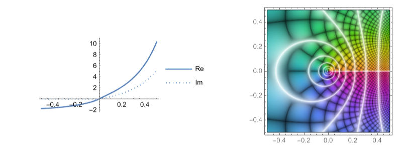
Plot them all together:
Going Back To Basics
Going Back To Basics
For comparison, this is the definition of the bilateral basic hypergeometric function:
Just as in the original bilateral case, there are three possible splittings, and thus three possible expressions for the bilateral basic hypergeometric function:
These are the corresponding functions:
As a numerical verification, we can look at some well-known special cases. For instance, here is Ramanujan's identity, a generalization of the Jacobi triple product:
This verifies one of Bailey’s bilateral summations:
Acknowledgments
Acknowledgments
I started drafting this note a few years ago, after some discussions with Tigran Ishkhanyan on implementing hypergeometric functions. This took longer than I would like to write, due to very spotty computer access, as well as health issues on my end. Hopefully, this note has helped make the bilateral hypergeometric function more useful.
CITE THIS NOTEBOOK
CITE THIS NOTEBOOK
On the bilateral hypergeometric function
by J. M.
Wolfram Community, STAFF PICKS, April 25, 2025
https://community.wolfram.com/groups/-/m/t/3450249
by J. M.
Wolfram Community, STAFF PICKS, April 25, 2025
https://community.wolfram.com/groups/-/m/t/3450249