ABSTRACT (original article): We present WI2easy, a Mathematica package for high-precision analysis of warm inflation (WI) dynamics, enabling efficient computation of both background evolution and curvature perturbations. Designed with a user-friendly interface, the tool supports a broad spectrum of inflaton potentials — including large-field, small-field, and hybrid models — and accommodates arbitrary dissipation coefficients dependent on temperature, field amplitude, or both, encompassing canonical forms prevalent in WI studies. Users can define custom models through intuitive commands, generating full dynamical trajectories and perturbation spectra in a streamlined workflow. This facilitates rapid confrontation of theoretical predictions with observational constraints, empowering systematic exploration of WI parameter spaces. WI2easy bridges the gap between theoretical models and observational cosmology, offering a robust, adaptable framework for next-generation inflationary analyses. CITATION (original article): Gabriel S. Rodrigues and Rudnei O. Ramos, WI2easy: warm inflation dynamics made easy, JCAP09(2025)014. https://doi.org/10.1088/1475-7516/2025/09/014
Model considered: , ,=100,Code options: radiation noise and thermalized inflaton perturbations
V(ϕ)=
V
0
4
M
Pl
4
ϕ
4
Υ(T,ϕ)=T
C
Υ
g
*
It is a good idea to start with a fresh kernel
Quit[]
Clean up leftover variables and start the kernel
ClearAll["Global`*"];
Move to the WI2easy directory through
SetDirectory[“<path to WI2easy main directory (where WI2easy.m is located)>”];
or if using directly this main.nb notebook, just run :
SetDirectory[“<path to WI2easy main directory (where WI2easy.m is located)>”];
or if using directly this main.nb notebook, just run :
In[]:=
SetDirectory[NotebookDirectory[]];
Load WI2easy
In[]:=
<<WI2easy.m
This is WI2easy v1.0
1. Definitions
1. Definitions
Parameters and model specific definitions (to be modified according to the model used) needed to run the code.
In[]:=
ParametersWI[]
You should get the following window
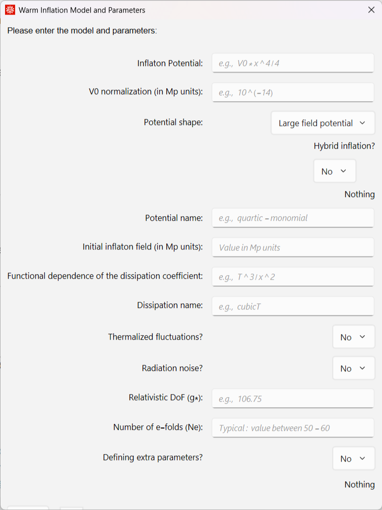
Run the command below to check the values you have given
pars
Out[]=
Potential,V0,PotentialTypequartic,HybridPotentialNO,InitialField25,DissipationT,DissipationTypeT,PotentialShape0,Thermalized1,RadNoise1,gstar100,Nefolds60,ExtraParamsNO
V0
4
x
4
1
100000000000000
Optional
Optional
The potential and dissipation function (along with all parameters), can also be defined here. These will overwrite any expressions given through the ParametersWI[] command
The inflaton potential V0* function of x : x = inflaton in Mp units
potential=V0*x^4/4;V0init=10^(-14);(*initialvalueforV0*)
Form of the dissipation coefficient : any function of T and x (do not include overall constant C_Upsilon)
funcdiss=T;
you can also define g_*, the radiation number of degrees of freedom here. In this example we will use g_ *= 100.
Define next any extra parameters that the model might require. There are no extra parameters required in this example.
gstar0=100;
2. Running the background equations and finding appropriate initial conditions
2. Running the background equations and finding appropriate initial conditions
Evolution of the background equations for a given range of dissipation ratio Q=Υ/(3H). It produces the initial conditions corresponding to a scale about k=10³ before Hubble radius crossing (which corresponds to about 7 e-folds before Hubble radius crossing, k=aH).
Use the command FindICs[Qi,Qf], giving the initial and final values of Q.
H
0
Use the command FindICs[Qi,Qf], giving the initial and final values of Q.
FindICs[10^(-9),4000]//AbsoluteTiming
Finding the ICs for Ntot= 60 efolds of inflation and for Q=1.×
-9
10
Out[]=
{1320.11,Null}
3. Running the perturbation (for the unnormalized spectrum) and generating data for G(Q)
3. Running the perturbation (for the unnormalized spectrum) and generating data for G(Q)
Evolution of the perturbation equations using the stochastic equations and obtaining the scalar power spectrum (in the φ = 0 gauge) from the Fokker-Planck equation. The data for the growth function G(Q) is obtained. Use the command FindGQ[] (with no arguments). It requires to first run FindICs[Qi,Qf] or to have the data file generated by FindICs.
(**********PerturbationsCode***********)(*SetDirectory[NotebookDirectory[]]SetOptions[OpenWrite,PageWidthInfinity];*)FindGQ[]//AbsoluteTiming
Finding now the value of G(Q) for Q=1.×
-9
10
Out[]=
{2472.88,Null}
4. Normalizing the spectrum and obtaining the observable quantities (for a single value of Q)
4. Normalizing the spectrum and obtaining the observable quantities (for a single value of Q)
Using the data for the growth function G(Q), the data is interpolated and the full scalar of curvature power spectrum is used to: normalize the spectrum with the COBE normalization and the observables (the tensor-to-scalar ratio r, spectral tilt and running ) are obtained for a given value of Q. Use the command ObservationsWI[Q,phi] given the values of Q and phi (in units of reduced Planck mass). It requires to first run FindICs[Qi,Qf] and then FindGQ[], or to have the data files generated by them.
n
s
α
s
ObservationsWI[1,7]//AbsoluteTiming
Running now spectrum code for Q=1..Finding the ICs for Ntot= 60 efolds of inflation and then normalizing the spectrum.
Running of main code for the observables: Successful.
epsilon(Nfinal)=1.00003 , spectrum(N_*)=2.10521× , C_Upsilon=0.0250809 , V_0=3.19972× , Q_*=1.02525 , r(N_*)=0.000337437 , ns(N_*)=0.968803 , alphas(N_*)=-0.000285172
-9
10
-15
10
Out[]=
{34.2288,{0.0250809,3.19972×,1.02525,0.000337437,0.968803,-0.000285172}}
-15
10
You can check the values of some key quantities here
Q_*=1.02525 , epsilon(Nfinal)=1.00003 , spectrum(N_*)=2.10521× , r(N_*)=0.000337437 , ns(N_*)=0.968803 , phi(N_*)/Mp= 10.6695 , Δϕ/Mp= 10.5307 , temp_end(GeV)= 5.64005× , N*= 58.137 , Ntot= 59.0794 , C_Upsilon= 0.0250809 , V0(GeV^4)= 1.12625× , V0/Mp^4= 3.19972× , V*(GeV^4)= 6.31584× , epsilonV*= 0.0702754 , etaV*= 0.105413 , V*^{1/4}/Mpl= 0.00179435 , T/H(N_*)= 122.633
-9
10
9
10
59
10
-15
10
70
10
Plotting background quantities : slow - row coefficient , Dissipation ratio Q, T/H, T, ϕ, equation of state, energy densities, all as a function of the number of efolds. The complete form of the spectrum is also generated
ϵ
H
MakePlotsEvolution
Making background plots for =1.
Q
*
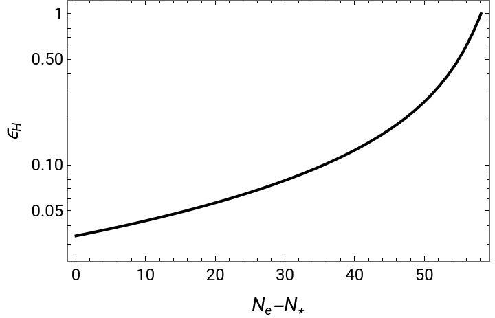
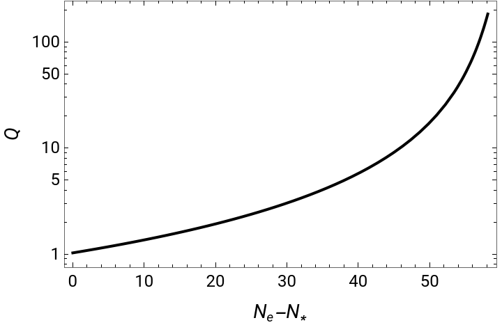
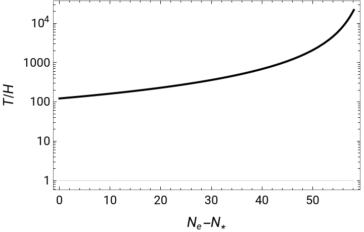
Obtain several background and perturbation quantities when the value of Q at Hubble crossing is varied. Use the command QrangeWI[Qinit] (with loop starting at the value Qinit). It requires to first run FindICs[Qi,Qf] and FindGQ[], or to have the data files generated by them. It generates background quantities (phi, \dot \phi, T/H, T/Mp, H, V0, CUpsilon, etc) and the observables (n_s, r, \alpha_s), all as a function of Q at Hubble crossing.
Plot additional quantities as a function of Q at Hubble crossing. It uses the data file generated from the previous part.
Data extracted from arXiv : 2110.00483
“BICEP/Keck XIII: Improved Constraints on Primordial Gravitational Waves using Planck, WMAP, and BICEP/Keck Observations through the 2018 Observing Season”, Figure 5
“BICEP/Keck XIII: Improved Constraints on Primordial Gravitational Waves using Planck, WMAP, and BICEP/Keck Observations through the 2018 Observing Season”, Figure 5
CITE THIS NOTEBOOK
CITE THIS NOTEBOOK
WI2easy: warm inflation dynamics made easy
by Gabriel S. Rodrigues and Rudnei O. Ramos
Wolfram Community, STAFF PICKS, March 31, 2026
https://community.wolfram.com/groups/-/m/t/3672541
by Gabriel S. Rodrigues and Rudnei O. Ramos
Wolfram Community, STAFF PICKS, March 31, 2026
https://community.wolfram.com/groups/-/m/t/3672541