Accurately modelling the passage of light through a system of lenses and other optical elements is important for many different areas in physics, computer graphics, and industry. I created a symbolic simulation of different optical systems using the Optica package and compared it to the output from its numerical ray tracing functionality. The symbolic simulation, once compiled, allows for fast iteration to optimize the system based on a given parameter.
This project uses the Optica package which can be be found at www.opticasoft.com.
This project uses the Optica package which can be be found at www.opticasoft.com.
Introduction
Introduction
Professional cameras can have over ten individual glass lens elements. This creates a system with a staggering number of variables such as each lens’s curvature and its separation from its neighbours. Optimizing this system numerically would be computationally costly and time-consuming. There is also the risk of any numerical optimization algorithm finding a local minimum for the system and not the global one. The Optica package has support for symbolic ray-tracing. This function takes in the initial coordinate of each ray and the parameters of the system (such as the focal length of the lenses) and outputs an expression for the final ray position on the screen as a function of these input parameters. Using this symbolic expression, I can quickly iterate through different components to modify the behaviour of the system. Optimization is simplified by expanding the symbolic expression as a Taylor series which allows the minimum to be found quickly numerically.
Needs["OpticaEM`OpticaEM`"];
Basic on-axis simulation using numerical and symbolic methods
Basic on-axis simulation using numerical and symbolic methods
I begin with a basic system of two plano-convex lens placed nearly end-to-end each with a focal length of 100 mm. In this example, I use the function to generate rays from a finite source. The rays from finite light source cannot be treated as parallel since they come from a source close to the optical system.
WedgeOfRays
Create a system with two plano-convex lenses
In[]:=
twoPlanoConvexExample = { Move[WedgeOfRays[10, WaveLength -> 0.4],{0,12.5,0}], WedgeOfRays[10, WaveLength -> 0.7], Move[PlanoConvexLens[{f1,100},50,9,CurvatureDirection->Back],90.5], Move[PlanoConvexLens[{f2,100},50,9],100.5],Move[Screen[{100,100}],205]};
Plot the system
In[]:=
TurboPlot[twoPlanoConvexExample, PlotType -> TopView, ImageSize -> 500,Frame -> True];
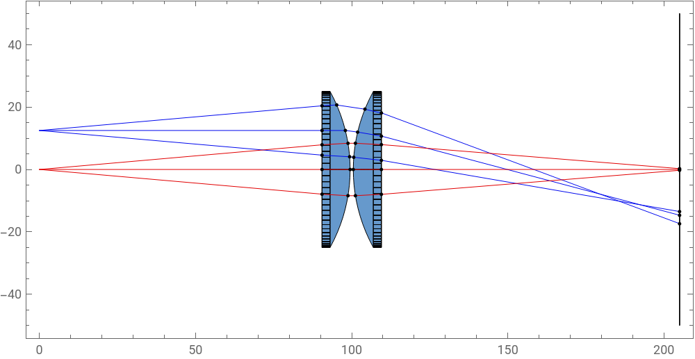
We can see that the focal surface of this system is not a plane at all (which would be ideal) but instead some form of curve. Light from finite sources increases the complexity of the simulation as it is not parallel to the optical axis of the system (off-axis). This makes simulation more complex by introducing a new angular dependence and increases the runtime of both numerical and symbolic methods. For these simple cases, I will only deal with on-axis light.
Create a system with two plano - convex lenses but only using a single ray
In[]:=
twoPlanoConvex = { Move[SingleRay[],{0,{x,0},{y,0}}], Move[PlanoConvexLens[{f1,100},50,9,CurvatureDirection->Back],90.5], Move[PlanoConvexLens[{f2,100},50,9],100.5], Move[Screen[{100,100}],205]};
The is a numerical function of all the ray paths as a function of the symbolic parameters I outlined for the system.
traceFunction
Trace rays through the whole system
In[]:=
traceFunction = RayTraceFunction/.TurboTrace[twoPlanoConvex, OutputType -> RayTraceFunction, EmbedRays -> True, ReportedParameters -> SurfaceCoordinates, ReportedSurfaces -> Last]
Out[]=
RayTraceFunction[{x, y, f1, f2}, -raytrace code: 4012040 Bytes- ]
This is the image I am going to send through the optical system. There is a lot of fine detail on the fur and in the grass which makes it easier to detect aberrations which might blur or distort these features.
In[]:=
dog =
;

To map the to the image, divides the image into pixels, calculates their origin, and traces an axial ray originating from this origin.
traceFunction
ProjectedPoints
Calculate the screen position of every pixel after propagation
In[]:=
ProjectedPoints[image_, xWidth_] := Module[{imageData, yDim, xDim, pDim, scale}, imageData = ImageData[image]; {yDim, xDim, pDim} = Dimensions[imageData]; scale = N[xWidth/xDim]; MapIndexed[ Function[{rgb, idx}, With[{y = idx[[1]], x = idx[[2]], sx = (idx[[2]] - xDim/2) * scale, sy = (idx[[1]] - yDim/2) * scale}, With[{proj = First[traceFunction[sx, sy, 100, 100]]}, {proj, rgb}]]], imageData, {2} ]];
In[]:=
numDog = ProjectedPoints[dog, 25];ColorPatchPlot[numDog, 25]
Out[]=
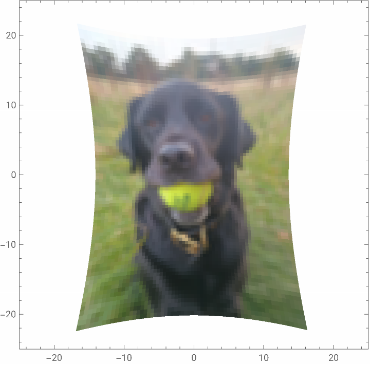
Images are reconstructed by dividing the screen into quadrilaterals with their corners defined by the rays from each pixel. The color of this polygon is the mean average of the four corner pixels. This is not a fully accurate representation of how a real image would appear because I am treating each ray as an unchanging delta function (x-,y-)when it is really convolved with the specific point spread function (PSF) of the optical system. This can and should be considered for more complex simulations.
δ
x
0
y
0
Interpolate between the projected pixels to recover the picture at the image plane
In[]:=
ColorPatchPlot[data_, width_] := Graphics[Flatten[#], PlotRange -> {{-width, width}, {-width, width}}, AspectRatio -> Automatic, Frame -> True]& @ Table[Module[{p1, p2, p3, p4, c1, c2, c3, c4, rgbList, avgColor}, {{p1, c1}, {p2, c2}, {p3, c3}, {p4, c4}} = {data[[i, j]], data[[i + 1, j]], data[[i + 1, j + 1]], data[[i, j + 1]]}; rgbList = List @@@ {c1, c2, c3, c4}; avgColor = RGBColor @@ Mean[rgbList]; {Polygon[{p1, p2, p3, p4}, VertexColors -> {avgColor, avgColor, avgColor, avgColor}]} ], {i, 1, Length[data] - 1}, {j, 1, Length[data[[1]]] - 1} ];
I then used the symbolic technique. returns the symbolic surface coordinates of the ray up to a second order polynomial expanded around the origin.
SymbolicTrace
Create a numerical function of the symbolic surface coordinates on the screen
In[]:=
N[symbolicCoords = (SymbolicSurfaceCoordinates /. SymbolicTrace[ twoPlanoConvex, {{y, 0, 2}, {x, 0, 2}, {f1 > 0, f2 > 0, x ∈ Reals, y ∈ Reals}}, MakeFloatingPoint -> True, Simplify -> False, RunningCommentary -> False, ReportedParameters -> {SymbolicSurfaceCoordinates}])];
In[]:=
ByteCount[symbolicCoords]
Out[]=
69820568
The is nearly 70 MB - this is a large function! In order to make it more manageable, we need to compile it.
ByteCount
In[]:=
CompiledFunc = Apply[Compile,{{x, y, f1, f2}, symbolicCoords}]
Out[]=
Project each pixel onto the screen using a symbolic function
In[]:=
ProjectedPointsSymbolic[image_, xWidth_, customFunc_] := Module[{imageData, yDim, xDim, pDim, scale}, imageData = ImageData[image]; {yDim, xDim, pDim} = Dimensions[imageData]; scale = N[xWidth/xDim]; MapIndexed[ Function[{rgb, idx}, With[{y = idx[[1]], x = idx[[2]], sx = (idx[[2]] - xDim/2) * scale, sy = (idx[[1]] - yDim/2) * scale}, With[{proj = customFunc[sx, sy, 100, 100]}, {proj, rgb}]]], imageData, {2} ]];
In[]:=
symDog = ProjectedPoints[dog, 25, CompiledFunc];ColorPatchPlot[symDog, 20]
Out[]=
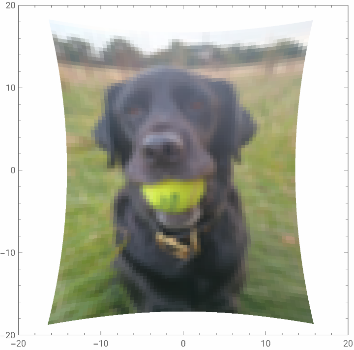
How do these two images compare? We can make a visualization by plotting the difference vectors between corresponding pixels.
Generate a vector plot of the difference in how two images are mapped by the optical system
We can see the deviation between the costlier but more accurate numerical simulation and the faster but more inexact symbolic simulation.
Chromatic aberration
Chromatic aberration
Chromatic aberration is also a feature of lenses due to the Sellmeier equation. Refraction is caused by the material’s response to the oscillating electric field of the photon as it passes through the material. This will vary (by different amounts for different materials) for different colors of light which will be focussed to different points. Chromatic aberration can be easily spotted in photographs there is a blue fringe on the outer edges of white regions.
I’ve defined a different optical system for each color wavelength. This is then compiled to a symbolic function as before.
I’ve defined a different optical system for each color wavelength. This is then compiled to a symbolic function as before.
Create new two plano-convex lens systems for different colors of light
Create symbolic functions for each color being traced through the system
This is a naive way of modelling chromatic aberration. In reality, every color of light will be shifted slightly, however, the majority of the spectral information about the image is lost when it is recorded so we only have the intensities of red, green, and blue light. The image is decomposed into these channels which are then
Decompose the image and project each color component through the system
Since each image is slightly shifted, we cannot add each set of pixels together. Instead, we rasterize the images and overlay them to retrieve the final aberrated image.
Concluding remarks
Concluding remarks
This project has answered several questions and raised several more. Firstly, we have seen that a symbolic representation of an optical system can be faster than a numerical simulation but the accuracy diminishes towards the extremes of the image as is expected for an expansion around the central point. For symbolic optimization, what is the best merit function to quantify the quality of the retrieved image? Although we only used a system of two plano-convex lens with two parameters (the focal lengths), the process took a long time to run on a consumer laptop. Is there a way to design simplify the symbolic equations to minimize their size so they don’t grow rapidly in size for more complex systems?
Lastly, treating rays as unchanging point particles is unphysical. The next stops are to include a way to calculate the point spread function at different areas of the lens.
Lastly, treating rays as unchanging point particles is unphysical. The next stops are to include a way to calculate the point spread function at different areas of the lens.
Acknowledgements
Acknowledgements
I have immensely enjoyed my time at Wolfram Summer School and I have learnt a tremendous amount about physics, Mathematica, and a lot of stuff which doesn’t fit into either category. I am very grateful to Piero Sanchez for his advice and help throughout this project and to Donald Barnhart for teaching me so much about Optica.
CITE THIS NOTEBOOK
CITE THIS NOTEBOOK
Symbolic modelling of optical systems
by Oliver Phillips
Wolfram Community, STAFF PICKS, July 9, 2025
https://community.wolfram.com/groups/-/m/t/3496156
by Oliver Phillips
Wolfram Community, STAFF PICKS, July 9, 2025
https://community.wolfram.com/groups/-/m/t/3496156