Don´t be afraid to do simple things
Robin Adams
The main goal of this book is to develop a basic conceptual understanding for the key aspects of modern Probabilistic Seismic Hazard Analysis (PSHA). The epigraph, which I picked up from Robin Adams, one of the pioneers of observational seismology in the 20th century, has stuck to my memory ever since I attended one of his training courses for young seismologists more than 30 years ago. It can be considered as one of the mottos for the approach taken here, namely to first develop concepts for rather simple situations in which most aspects are easy to understand. Subsequently, these concepts can be extended to more realistic situations. It has been my experience that this transition from the “toy world” to the “real world” can at least partially done rather intuitively.
Probabilistic seismic hazard analysis (PSHA) deals with probabilistic models for seismically generated ground motion and the assessment of the corresponding uncertainties. It draws from a number of disciplines such as probability theory, earthquake seismology and earthquake engineering. The fact that the analysis of any type of natural hazard is concerned with situations which are characterized by large amounts of uncertainties and randomness makes uncertainty assessment a key element of hazard analysis. In the context of seismic hazard it is for example the spatial distribution of future earthquakes which is uncertain, as are their occurrence rates, their source properties, and their site specific shaking characteristics. As a consequence, modern probabilistic seismic hazard analysis (PSHA) is usually accompanied by a systematic uncertainty analysis, sometimes involving different experts or expert groups. Different experts might provide different estimates for the building blocks of a hazard model, which in themselves carry uncertainties. In other words, uncertainties are everywhere and they appear in different flavors. Uncertainties are called aleatory (from alea the Latin word for dice) if they appear as an intrinsic and inseparable aspect of the process under study. They are referred to as epistemic (from the Greek word ϵπιστϵμωσ related to knowledge) if they are caused simply from the lack of knowledge. Epistemic uncertainties can be reduced, at least in principle, by gathering more knowledge while aleatory can not. This makes important differences for the way these can be treated in practice.
Some aspects of the process under consideration might also be more uncertain than others, independent on the type of uncertainty. This naturally leads to the need for the quantification of different degrees of uncertainties. A common way in which this is done is in terms of probabilities. As a consequence, before we even start to think about details of a seismic hazard model in terms of seismicity models, earthquake source properties, site effects, or how to calculate hazard curves, we have to make sure that we have a basic knowledge in probability theory. This will be covered in chapter 2.
Fundamental aspects of earthquake seismology and earthquake engineering are very briefly touched upon in chapters 3 and 4, respectively, but only to a degree which I consider necessary from a seismic hazard analysis perspective. This is then covered in detail in chapter 5, which presents the derivation of hazard curves, one of the key outputs of any PSHA, from multiple perspectives, offering both theoretical and practical insights. From a probability-theoretical standpoint, ground motion can be treated as a random variable (RV) with hazard curves serving as one of many ways to represent its distribution function. Alternatively, from a more pragmatic perspective, hazard curves will be viewed as the outcome of a fictitious long-term observational process. By assuming nature to be consistently observable over extended periods, one can track how frequently certain ground motion levels are exceeded, essentially treating hazard analysis as a systematic bookkeeping exercise. Chapter 5 introduces these and other viewpoints, aiming to provide at least one approach that resonates with every reader. The discussion is kept concise, allowing the material to serve as the foundation for a “crash course” that can be covered in just a few days.
Full book: Frank Scherbaum, “Fundamental Concepts of Probabilistic Seismic Hazard Analysis” from the Notebook Archive (2025), https://notebookarchive.org/2025-02-5zwyxr9
The following is a sample of Chapter 3 from the book. The full code for Chapter 3 is provided at the end.
3
. Earthquake Seismology Primer for PSHAWhen the earth shakes, the foundations of human arrogance are tested.
Seneca
Probabilistic seismic hazard analysis draws from a number of different fields of science, one of the most obvious being earthquake seismology. Earthquakes are the cause of the seismic hazard but it does not hurt to remind us again and again that what constitutes the actual threats are effects of earthquakes such as strong ground shaking or tsunamis, not the earthquakes themselves. Here we will concentrate on the shaking hazard. In this chapter I will touch upon those aspects of earthquake physics, wave propagation and site effects, which are needed to understand the essential building blocks of probabilistic seismic hazard models at a very basic level. More advanced aspects are covered in the second part of this book.
3.1. The earthquake source
3
.1
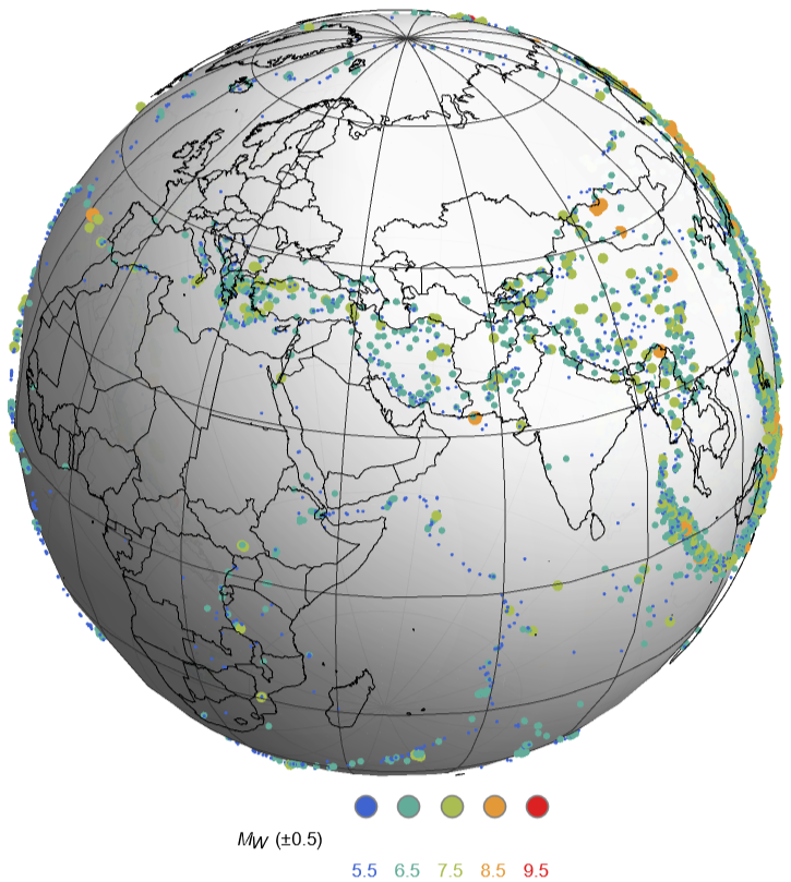
. The earthquake sourceFig. 3.1.1 shows the global distribution of potentially damaging earthquakes from 1900 to 2009, color coded according to earthquake strength (magnitude). What is immediately obvious from Fig. 3.1.1 is that the spatial distribution of these earthquakes is highly non-uniform.
Figure
3
.1
.1 Global distribution of earthquakes from 1900-2009. Data source: ISC-GEM catalog (Storchak et a., 2013). You can turn the globe using the mouse.Fig. 3.1.2 shows the same set of earthquake locations in map view. The non-uniform spatial distribution becomes even more obvious if the earthquake hypocenters (the locations at which the earthquake ruptures start) are separated into different depth ranges (shallow, intermediate, deep). In particular the intermediate and deep earthquakes (panels Intermediate and Deep in Fig. 3.1.2) are spatially concentrated. The dominant features of the spatial pattern of earthquakes can easily be understood within the scientific theory of plate tectonics (see e. g. Press and Siever, 1986). Most seismic energy is released where tectonic plates (which move relative to each other at speeds of up to a few cm/year) meet. These regions are called plate boundaries. It is actually not surprising that the plate boundaries coincide with the regions of concentrated seismicity (panel Plate Boundaries in Fig. 3.1.2) since the spatial distribution of seismicity was an important piece of information for the definition of plate boundaries.
All
Shallow
Intermediate
Deep
Plate Boundaries
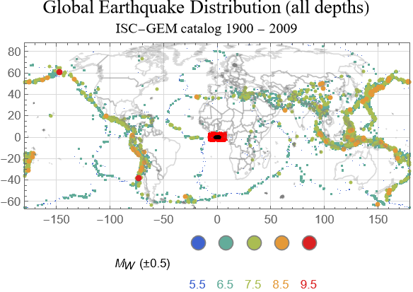
Figure 3.1.2 Global distribution of earthquake epicenters (projections of the hypocenters to the surface) from 1900-2009. You can select different depth ranges for display. Data source: ISC-GEM catalog (Storchak et a., 2013). Plate boundaries after DeMets et al. (2010). Plate name abbreviations: AM, Amur; AN, Antarctica; AR, Arabia; AU, Australia; CA, Caribbean; CO, Cocos; CP, Capricorn; CR, Caroline; EU, Eurasia; IN, India; LW, Lwandle; NA, North America; NB, Nubia; NZ, Nazca; OK, Okhotsk; PA, Pacific; PS, Philippine Sea; SA, South America; SC, Scotia; SM, Somalia; SR, Sur; SU, Sundaland; SW, Sandwich; YZ, Yangtze.
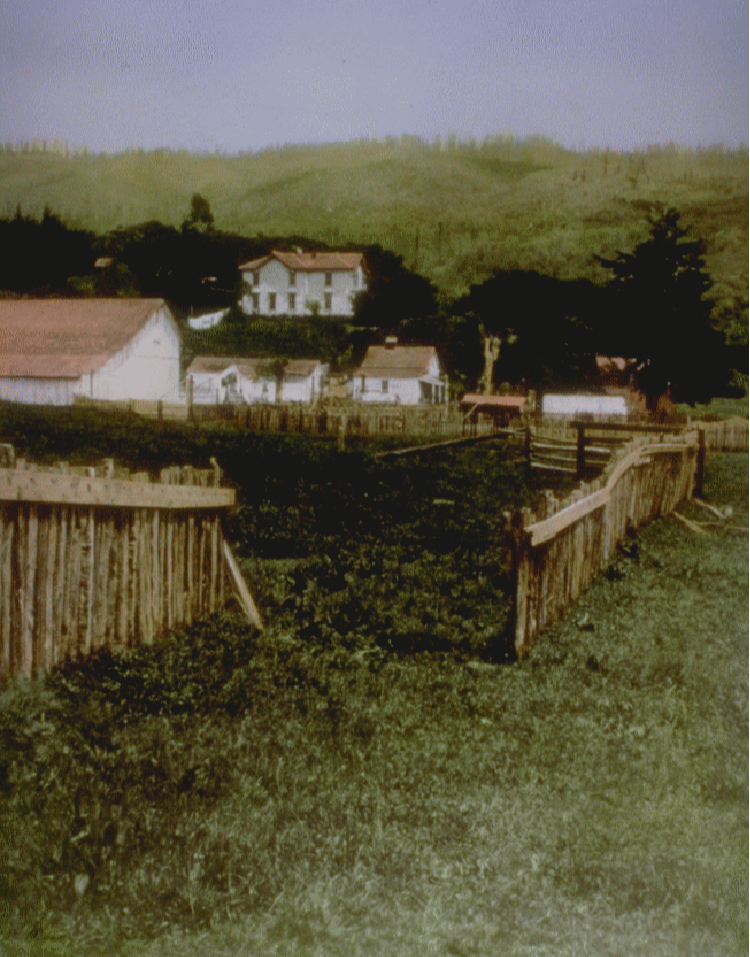
The physical mechanisms behind the processes during individual earthquakes have been enigmatic up to not very long ago. Over the course of human history, most cultures have developed their own myths to explain the generation of earthquakes, mostly involving different kinds of animals. It was a single event at the beginning of the last century, the San Francisco earthquake of April 18, 1906, which has paved the way for our current understanding of earthquake physics. One of the most remarkable observations during that earthquake was that of of large horizontal ground dislocations, as for example documented in Fig. 3.1.3.
Figure
3
.1
.3 This picture shows a fence near Woodville in California that was offset by 2.6 m during the the San Francisco earthquake of 18 April 1906. The photo was taken at Lat: 36,106, Lon: -119,199 and is looking northeast. Image source: NOAA/NGDC, G.K. Gilbert, U.S. Geological Survey. Photo has been colorized.The analysis in the aftermath of this earthquake by Henry Fielding Reid of Johns Hopkins University has led to what is now called elastic rebound theory (Reid, 1910). In a nutshell, the elastic rebound theory sees earthquakes as shear ruptures driven by previously stored elastic energy. Before an earthquake, the ground deforms in reaction to plate tectonic forces and deformation energy is stored in the rock volume surrounding the later hypocenter. Over time, deformation increases until the shear strength of the rock (or the frictional resistance of the fault which is going to rupture) is reached and the rupture starts. During the rupture process, part of the stored deformation energy is released in form of seismic wave energy and the accumulated stress is at least partially released. Subsequently, the process can start over. Fig. 3.1.4 illustrates the key aspects of the rupture phase and the initiation of the radiation of seismic waves.
Figure
3
.1
.4 The rupture phase of an earthquake. The Mathematica code to create this figure is from the blogpost by Yu-Sung Chang from Wolfram research (Chang, 2013; posted March 18, 2013). Plate boundaries are the regions where most of the seismic energy is released on a global scale. However, although visible in Fig. 3.1.1 and Fig. 3.1.2 only at second glance (e. g. in Australia), it needs to be emphasized that the interior of tectonic plates is not free of earthquakes. Intraplate earthquakes, earthquakes which occur at considerable distances away from plate boundaries are called, are not restricted to small magnitudes and can pose considerable hazard (Johnston and Kanter, 1990). Famous historical example are provided by the New Madrid earthquake sequence in the winter of 1811/12 with three earthquakes of magnitude all larger than 7.5 (Johnston and Schweig, 1996).
3.1.1. Styles of faulting
3
.1
.1
. Styles of faultingDuring the rupture phase of an earthquake, strained blocks of rock material rapidly move against each other on what is usually approximated as a planar surface referred to as fault plane. In Fig. 3.1.4 the fault plane would be oriented vertically. If you imagine yourself standing close to the boundary of one of the two moving blocks and look at the opposite block, it would move to the left relative to your position. For this to apply it does not matter on which side of the fault your are standing. Such a sense of relative motion of the two blocks would be called left-lateral. If the other block would move to the right relative to your position, the sense of motion would be called right lateral. It is the relative motion of the block on the other side that defines the sense. Since the motion in Fig. 3.1.4 is purely horizontal, the mechanism would be called a “left-lateral horizontal strike slip motion”.
Exercise
3
.1
.1 Is the sense of motion in Fig. 3.1.4 left-lateral or right-lateral?In general, fault planes can be tilted and the relative motion of the block of rock material which move against each other can take arbitrary angles with respect to the horizontal direction. This leads to different styles of faulting some of which are illustrated in Fig. 3.1.5.
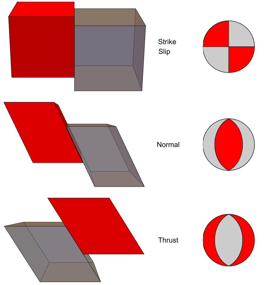
The type of mechanism that develops during faulting depends on the orientation of the fault plane with respect to the orientation of the acting stresses, which would fully be described by a quantity called the stress tensor or in simpler terms by the orientation and magnitude of three force vectors (P-, B-, and T-axis) which are oriented perpendicular to each other. In Fig 3.1.6 the different styles of faulting are illustrated in dependence of the values of the strike direction (ϕ) of the fault plane clockwise against geographic North, the dip angle (δ) of the fault plane against the surface of the Earth, and the slip angle(λ) of the so-called hanging block (orange) against the foot wall block (white), respectively. Several classification schemes have been proposed in the literature. For a comparison of different definitions see Table 1 in Bommer et al. (2003). Here, for the classification of the fault types into thrust faulting, normal faulting, strike slip faulting, the scheme by Frohlich and Apperson (1992) is used. The P- and T- axis denote the local pressure and tension axis during faulting. U denotes the slip direction of the hanging block. δP, δT, and δB are the so-called plunge angles of the P-, T-, and neutral axis against the horizontal, respectively.
With a few exceptions, such as e. g. the Swabian Jura region in SW Germany where essentially all recorded earthquakes show left-lateral strike slip faulting, the styles of faulting in a seismically active region usually show considerable variation between different earthquakes. However, a certain style of faulting, the type of which depends on the tectonic situation, is often observed to be dominant. In compressional regimes for example, one would expect to have a larger propensity towards thrust faulting where one block, the hanging wall, is moved on top of the other, the foot wall, than in extensional regime where normal faults, the hanging wall is sliding down on top of the foot wall, are more likely.
What is important in the context of seismic hazard analysis is the observation that the average ground motion level to be generated from an earthquake of a certain magnitude systematically changes with the style of faulting. Normal faults for example tend to produce lower average levels of ground shaking than thrust faults. This will be discussed in much more detail later.
During an earthquake, part of the energy which is stored within the deformed crustal volume surrounding the rupturing fault is released in form of seismic waves, which propagate away from the earthquake and, depending on their energy and frequency content, can cause damage to buildings. The interaction of seismic waves with man-made structures is discussed in chapter 4. The purpose of the present section is to introduce the fundamental aspects of the generation and propagation of seismic waves. In the context of PSHA, we have to be aware of the different types of waves that can be generated from an earthquake and of some of their elementary properties. Let´s start with a simple exercise.
In the context of seismic waves, one can distinguish different wave types, which differ in the boundary conditions under which they develop and in the way they propagate with respect to the particle motion they cause.
Surface waves, as implied by their name, are waves that propagate close to the surface of the Earth and their amplitude diminishes rapidly with depth. Depending on to their polarization properties they are either called Love waves after the A. E. H. Love, or Rayleigh waves after Lord Rayleigh. Love waves (Fig. 3.2.5) are horizontally polarized and result from the interaction of horizontally polarized shear waves (so-called SH waves) in a layered medium.
The second type of surface waves, Rayleigh waves (Fig. 3.2.6-3.2.7), are combination of compressional waves and vertically polarized shear waves, so-called SV waves. In contrast to Love waves, they can also exist along a homogeneous half-space (without any layering). The polarization of Rayleigh waves is in general elliptic which means each particle affected by Rayleigh waves propagates along an elliptical trajectory (usually retrograde with respect to the wave propagation direction).
Another property, which distinguishes surface waves from body waves is the fact that their wave speed can become a function of frequency if they propagate in layered media. The dispersion is called normal if the low frequency components of the waves propagate faster than the high frequency components. In terms of shaking characteristics this means that the initial shaking will have lower frequencies than the later parts.
The spatially anisotropic deformation pattern which develops in the immediate vicinity of an earthquake during the rupture process as illustrated in Fig. 3.1.7 has an important consequence for the radiation of seismic energy in the form of seismic waves. In contrast to explosion sources, where the radiation of seismic energy is (ideally) only in form of compressional seismic waves (P-waves) and is radially symmetric with respect to the hypocenter, the radiation of seismic energy from earthquakes is in form of P- and S- waves and spatially anisotropic. This is illustrated in Fig. 3.2.8 for compressional (P-) waves, shear (S-) waves in general, vertically polarized shear (SV) waves, and horizontally polarized shear (SH) waves. For this illustration, the earthquake source is approximated by a so-called double-couple point source (for details see e. g. Aki and Richards, 2002) of arbitrary orientation in three dimensions. You can define the the strike direction (ϕ) of the fault, the dip angle (δ) of the fault plane against the surface of the Earth, and the slip angle(λ) of the hanging block against the foot wall block as well as the wave type.
In addition to the spatially anisotropic radiation pattern caused by the deformation pattern within the source volume, the fact that the rupture front itself propagates with a finite speed (most often less than the shear wave speed) along the fault also causes directional dependence of the radiated waves due to the Doppler effect (Fig. 3.2.9).
An observer in the direction in which the sources is moving will observe higher frequencies than an observer behind the source.
References
References
Aki, K. and P. Richards (2002). Quantitative Seismology, 2nd ed. , University Science Books, Sausalito, California.
Anderson, J. A. , and H.O. Wood (1925). Description and theory of the torsion seismometer., Bulletin of the Seismological Society of America, 15, 1-72.
Atkinson, G. M. (2006) Single-station sigma, Bulletin of the Seismological Society of America 96(2) , 446-455.
Bommer, J. J., A. Douglas, and F. O. Strasser (2003). Style-of-faulting in ground motion prediction equations, Bulletin of Earthquake Engineering, 1(2), 171-203.
Boore, D. M. , and W. B. Joyner (1997). Site amplifications for generic rock sites, Bulletin of the Seismological Society of America, 87(2), 327-341.
Boore, D. M. (2003). Simulation of ground motion using the stochastic method, Pure and Applied Geophysics, 160, 635-676.
Boore, David M. , and Gail M. Atkinson (2008). Ground-Motion Prediction Equations for the Average Horizontal Component of PGA, PGV, and 5%-Damped PSA at Spectral Periods between 0.01 s and 10.0 s, Earthquake Spectra, 24(1), 99-138.
Bormann, P. (Ed.) (2012). New Manual of Seismological Observatory Practice (NMSOP-2), IASPEI, GFZ German Research Centre for Geosciences, Potsdam; http://nmsop.gfz-potsdam.de; DOI: 10.2312/GFZ.NMSOP-2.:urn:nbn:de:kobv:b103-NMSOP-2
Chang, Y., 2013, Built to last: Understanding Earthquake engineering. http://blog.wolfram.com/2011/03/18/built-to-last-understanding-earthquake-engineering/
Cotton, Fabrice, Ralph Archuleta, and Mathieu Causse (2013). What is Sigma of the Stress Drop?, Seismological Research Letters, 84(1), 42-48.
DeMets, C., Gordon, R. G., and Argus, D. F., 2010. Geologically current plate motions, Geophysical Journal International , v. 181, no. 1, p. 1-80.
Frohlich, C. , and K. D. Apperson (1992). Earthquake focal mechanisms, moment tensors, and the consistency of seismic activity near plate boundaries, Tectonics, 11(2), 279-296.
Fukushima, Yoshimitsu (1996). Scaling relations for strong ground motion prediction models with M (super 2) terms, Bulletin of the Seismological Society of America, 86(2), 329-336.
Grünthal G (ed) (1998) European Macroseismic Scale 1998. Cahiers du Centre Europèen de Gèodynamique et de Seismologie. Conseil de l’Europe, Conseil de l’Europe.
Gutenberg, B. , and C. F. Richter (1942). Earthquake magnitude, intensity, energy, and acceleration, Bulletin of the Seismological Society of America, 32, 163-191.
Gutenberg, B. , and C.F. Richter (1956). Earthquake magnitude, intensity, energy, and acceleration (second paper), Bulletin of the Seismological Society of America, 46(2), 105-145.
Hanks, T. C. , and H. Kanamori (1979). A moment magnitude scale, Journal of Geophysical Research, 84(B5), 2348-2350.
Havskov, J. , and L. Ottemöller. (2010). Routine Data Processing in Earthquake Seismology: Springer Dordrecht Heidelberg London New York.
Johnston, A. C., and L. R. Kanter, Earthquakes in stable continental crust, Sci. Am., 262(3), 68-75, 1990.
Johnston, A.C., and Schweig, E.S., 1996, The enigma of the New Madrid earthquakes of 1811-1812: Annual Review of Earth and Planetary Sciences, v. 24, p. 339-384; doi: 10.1146/annurev.earth.24.1.339;
Joyner, W. B. and D. M. Boore (1981). Peak horizontal acceleration and velocity from strong-motion records including records from the 1979 Imperial Valley, California, earthquake, Bull Seism. Soc. Am. 71, 2011-2038.
Leydecker, G. (2011): Erdbebenkatalog für Deutschland mit Randgebieten für die Jahre 800 - 2008 (Earthquake catalogue for Germany and adjacent areas for the years 800 to 2008). – Geol. Jb., E 59; 198 S., 12 Abb., 5 Tab., 9 Anhänge, 1 CD; BGR Hannover; Vertrieb: E. Schweizerbart’sche Verlagsbuchhandlung, Stuttgart.
McGuire, R. K. (2004). Seismic hazard and risk analysis (Vol. MNO-10): Earthquake Engineering Research Institute.
Musson, R. M. W., G. Gruenthal, and M. Stucchi (2010). The comparison of macroseismic scales, Journal of Seismology, 14, 413-428.
Power, Maurice, Brian Chiou, Norman Abrahamson, Yousef Bozorgnia, Thomas Shantz, and Clifford Roblee (2008). An Overview of the NGA Project, Earthquake Spectra, 24(1), 3-21.
Press, F., and R. Siever, Earth, 4th edition, Freeman and Co., New York, NY, 656 pp., hardcover, 1986
Reid, H.F., The Mechanics of the Earthquake, The California Earthquake of April 18, 1906, Report of the State Investigation Commission, Vol.2, Carnegie Institution of Washington, Washington, D.C. 1910 (see especially pages 16-28).
Richter, C. F. (1935). An instrumental earthquake magnitude scale., Bulletin of the Seismological Society of America, 25, 1-32.
Somerville, P. and J. Yoshimura (1990), The influence of critical Moho Reflections on strong ground motions recorded in San Francisco and Oakland during the 1989 Loma Prieta Earthquake, Geophys. Res. Letters, 17(8), 1203–1206.
Stevens, S. S. (1946). On the theory of scales of measurement, Science, 103(2684), 677-680.
Storchak, D.A., D. Di Giacomo, I. Bondár, E. R. Engdahl, J. Harris, W.H.K. Lee, A. Villaseñor and P. Bormann. Public Release of the ISC-GEM Global Instrumental Earthquake Catalogue (1900- 2009), subm. to Seismological Research Letters, 2013.
Wald, D. J., V. Quitoriano, T. Heaton, H. Kanamori, C. W. Scrivner, and B. C. Worden (1999). TriNet ``ShakeMaps’’: Rapid Generation of Instrumental Ground Motion and Intensity Maps for Earthquakes in Southern California, Earthquake Spectra, 15(3), 537-556.
Youngs, R. B. , and K. J. Coppersmith (1985). Implications of fault slip rates and earthquake recurrence models to probabilistic seismic hazard estimates, Bulletin of the Seismological Society of America, 75(4), 939-964.
Related Demonstrations
Related Demonstrations
"Deformation Pattern in an Earthquake Source Region" from the Wolfram Demonstrations Project
http://demonstrations.wolfram.com/DeformationPatternInAnEarthquakeSourceRegion/
http://demonstrations.wolfram.com/DeformationPatternInAnEarthquakeSourceRegion/
"Styles of Faulting" from the Wolfram Demonstrations Project
http://demonstrations.wolfram.com/StylesOfFaulting/
http://demonstrations.wolfram.com/StylesOfFaulting/
"Earthquake Focal Mechanism" from the Wolfram Demonstrations Project
http://demonstrations.wolfram.com/EarthquakeFocalMechanism/
http://demonstrations.wolfram.com/EarthquakeFocalMechanism/
Full code for Chapter 3
CITE THIS NOTEBOOK
CITE THIS NOTEBOOK
Fundamental concepts of probabilistic seismic hazard analysis
by Frank Scherbaum
Wolfram Community, STAFF PICKS, March 26, 2025
https://community.wolfram.com/groups/-/m/t/3433224
by Frank Scherbaum
Wolfram Community, STAFF PICKS, March 26, 2025
https://community.wolfram.com/groups/-/m/t/3433224