This notebook contains the underlying computational analysis of a recent open-access publication in PNAS, Peak grain forecasts for the US High Plains amid withering waters. It is a representation of groundwater use–crop production dynamics across three High Plains states of Kansas, Nebraska, and Texas.
Crop statistics
Survey Data
Survey Data
Combining Northern and Southern High Plains data from the USDA National Agricultural Statistics Service query tool (Access January 2020)
Combining Northern and Southern High Plains data from the USDA National Agricultural Statistics Service query tool (Access January 2020)
I have downloaded data for 4 crops: cotton, corn, sorghum, and wheat. On the USDA NASS query tool, I chose to retrieve data for two Texas agricultural districts of interest: the northern and southern High Plains agricultural districts.
Import
Import
In[]:=
Directory[]
Out[]=
C:\Users\mrada\Documents
In[]:=
SetDirectory["C:\\Users\\mrada\\Google Drive\\Research projects\\Peak Water\\Texas"]
Out[]=
C:\Users\mrada\Google Drive\Research projects\Peak Water\Texas
In[]:=
surveyDataset=Import["Sheets\\By Agricultural District\\cotton_corn_sorghum_wheat.csv","Dataset","HeaderLines"1];
Show keys
Show keys
In[]:=
Normal@Keys@surveyDataset〚1〛
Out[]=
{Program,Year,Period,Week Ending,Geo Level,State,State ANSI,Ag District,Ag District Code,County,County ANSI,Zip Code,Region,watershed_code,Watershed,Commodity,Data Item,Domain,Domain Category,Value,CV (%)}
Show data items
Show data items
In[]:=
Normal@DeleteDuplicates@surveyDataset[All,"Data Item"]
Out[]=
{CORN, GRAIN, IRRIGATED - PRODUCTION, MEASURED IN BU,CORN, IRRIGATED - ACRES PLANTED,COTTON, UPLAND, IRRIGATED - ACRES PLANTED,COTTON, UPLAND, IRRIGATED - PRODUCTION, MEASURED IN 480 LB BALES,SORGHUM, GRAIN, IRRIGATED - PRODUCTION, MEASURED IN BU,SORGHUM, IRRIGATED - ACRES PLANTED,WHEAT, WINTER, IRRIGATED - ACRES PLANTED,WHEAT, WINTER, IRRIGATED - PRODUCTION, MEASURED IN BU}
Show earliest and latest data point for each data item
Show earliest and latest data point for each data item
In[]:=
surveyDataset[GroupBy[#["Data Item"]&],{Min[#],Max[#]}&,"Year"]
Out[]=
Corn data only exists for after 1981 compared to the early 1970s for the other three crops. We will need to supplement the data for corn using separate data sources. This will be done below.
For which years does survey data exist for all four crops?
For which years does survey data exist for all four crops?
In[]:=
fourCropYears=Intersection@@Normal@surveyDataset[GroupBy[#["Data Item"]&],All,"Year"]
Out[]=
{1981,1982,1983,1984,1985,1986,1987,1988,1989,1990,1991,1992,1993,1994,1995,1996,1997,1998,1999,2000,2001,2002,2003,2004,2005,2006,2007,2009,2010,2012,2015,2016,2017}
Create a dataset containing only the years where data for the four crops exists.
Create a dataset containing only the years where data for the four crops exists.
In[]:=
cropDataset=surveyDataset[Select[MemberQ[fourCropYears,#["Year"]]&]];
For each year, sum the weight of crops produced (be careful of units!) and the acres planted
For each year, sum the weight of crops produced (be careful of units!) and the acres planted
Give values appropriate units: weights in metric tons and areas in hectars. Be mindful that 1 bushel of corn and sorghum are 56 lbs but 1 bushel of winter wheat is 60 lb (link)
In[]:=
cropDatasetUnit=cropDataset[All,Association[#,"Value"Which[StringMatchQ[#["Data Item"],___~~"ACRES"~~___],N[Quantity[#["Value"],"Acres"]~UnitConvert~"hectares"],StringMatchQ[#["Data Item"],___~~"CORN"~~___~~"PRODUCTION"~~___],N[Quantity[#["Value"]*56,"lb"]~UnitConvert~"metric tons"],StringMatchQ[#["Data Item"],___~~"SORGHUM"~~___~~"PRODUCTION"~~___],N[Quantity[#["Value"]*56,"lb"]~UnitConvert~"metric tons"],StringMatchQ[#["Data Item"],___~~"WHEAT"~~___~~"PRODUCTION"~~___],N[Quantity[#["Value"]*60,"lb"]~UnitConvert~"metric tons"],StringMatchQ[#["Data Item"],___~~"COTTON"~~___~~"PRODUCTION"~~___],N[Quantity[#["Value"]*480,"lb"]~UnitConvert~"metric tons"]]]&];
Sum weights and areas per year
Sum weights and areas per year
In[]:=
cropDatasetUnitGrouped=cropDatasetUnit[GroupBy[#["Year"]&],GroupBy[QuantityUnit[#["Value"]]&],Total,#["Value"]&][All,<|"Production""MetricTons","Area""Hectares"|>];
Add census data for all four crops in 1959, 1964, and corn irrigated acreage in 1974 and 1978
Add census data for all four crops in 1959, 1964, and corn irrigated acreage in 1974 and 1978
The USDA data we extracted above were survey data which apparently only started in the 1970s for a lot of the crops and only in the 1980s for corn, probably because corn wasn’t as popular back then (as we will see below). However, there are census data from even before. For example, if you play around the USDA website, you will be able to find census data containing harvested irrigated crop by county in Texas for 1964 and 1959 (link). This will be used to supplement data for all four crops considered here. We still need census data for corn in 1974 (link) and 1978 (link). The first unfortunate characteristic of these censuses is that they are in pdf in low quality. This means I had to manually go through each county and copy the data to an excel sheet to make it convenient to analyze here. Moreover, for 1974 and 1978, there are only data on the amount of acres of irrigated corn, not production. We will then need to estimate the yield of irrigated corn in the Texas northern and souther High Plains districts. Yield is expressed in Bushels (unit of weight) per Acre so by multiplying the acreage (data we have) by the yield, we obtain the production in Bushels.
Estimate Texas irrigated corn yields by agricultural district and obtain production estimates
Estimate Texas irrigated corn yields by agricultural district and obtain production estimates
Import Kansas irrigated corn yields from downloaded excel sheet
Import Kansas irrigated corn yields from downloaded excel sheet
Irrigated corn yield in Kansas (in Bushels/acre )
In[]:=
kansasCornYieldDataset=Import["Sheets\\corn_yield_kansas_texas.csv","Dataset","HeaderLines"1][Select[StringMatchQ[#["State"],"KANSAS"]&]];
Import Texas irrigated corn yields from downloaded excel sheet for the two districts
Import Texas irrigated corn yields from downloaded excel sheet for the two districts
Irrigated corn yield in Texas (in Bushels/acre )
In[]:=
texasCornYieldDataset=Import["Sheets\\corn_yield_texas_agdistrict.csv","Dataset","HeaderLines"1];
Show Keys
In[]:=
Normal@Keys@texasCornYieldDataset〚1〛
Out[]=
{Program,Year,Period,Week Ending,Geo Level,State,State ANSI,Ag District,Ag District Code,County,County ANSI,Zip Code,Region,watershed_code,Watershed,Commodity,Data Item,Domain,Domain Category,Value,CV (%)}
Show Ag Districts
In[]:=
Normal@DeleteDuplicates@texasCornYieldDataset〚All,"Ag District"〛
Out[]=
{NORTHERN HIGH PLAINS,SOUTHERN HIGH PLAINS}
Compare Texas northern and southern districts to Kansas irrigated corn yields
Compare Texas northern and southern districts to Kansas irrigated corn yields
In[]:=
ListPlot[{kansasCornYieldDataset[All,{"Year","Value"}],texasCornYieldDataset[Select[StringMatchQ[#["Ag District"],"NORTHERN HIGH PLAINS"]&],{"Year","Value"}],texasCornYieldDataset[Select[StringMatchQ[#["Ag District"],"SOUTHERN HIGH PLAINS"]&],{"Year","Value"}]},PlotRange{{1970,1990},{0,170}},AxesLabel{"Year","Corn Yield (BU/Acre)"},PlotLegends{"Kansas","Texas northern district","Texas southern district"},FillingBottom]
Out[]=
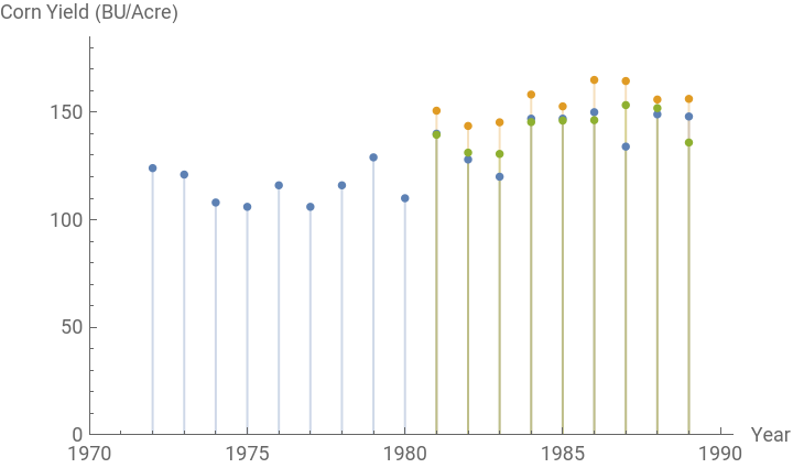


We need to estimate Texas irrigated corn yields prior to 1981 using the Kansas yields. We first compute the ratios of yields between Texas north and south High Plains agricultural districts to Kansas’ after 1980:
For the northern district
In[]:=
Normal@texasCornYieldDataset[Select[StringMatchQ[#["Ag District"],"NORTHERN HIGH PLAINS"]&],"Value"]/Normal@kansasCornYieldDataset[Select[#["Year"]>1980&],"Value"]
Out[]=
1.05541,1.04631,1.22761,,1.03878,1.07619,1.21083,1.12188,1.07643
11
10
In[]:=
{Mean@#,StandardDeviation@#}&@%
Out[]=
{1.10594,0.0693474}
For the southern district
In[]:=
Normal@texasCornYieldDataset[Select[StringMatchQ[#["Ag District"],"SOUTHERN HIGH PLAINS"]&],"Value"]/Normal@kansasCornYieldDataset[Select[#["Year"]>1980&],"Value"]
Out[]=
{0.918243,1.01946,1.14403,0.975333,0.993878,0.989116,1.08833,1.025,0.996429}
We notice that the standard deviations of the ratios is two order of magnitudes smaller that the mean of the ratios. Based on these results, multiply Kansas yields in 1974 and 1978 by 1.11 (11%) to estimate the Texas northern district irrigated corn yield and 1.02 (2%) for southern district.
Import corn irrigated acreage for Texas. These are to be multiplied by the estimated yields to obtain production values.
Import corn irrigated acreage for Texas. These are to be multiplied by the estimated yields to obtain production values.
We import an excel sheet that I have manually created based on the pdf files of the census (find the online links above).
Missing data is denoted by an empty string (“”). We want to be able to refer to a certain data point using the year, so we make the YEAR column a set of keys as follows:
Obtain irrigated corn production estimates for the Texas High Plains in 1978
Obtain irrigated corn production estimates for the Texas High Plains in 1978
1978
Assume that missing data means that irrigated acreage is 0.
1974
Assume that missing data means that irrigated acreage is 0.
Add irrigated corn census data to the irrigated survey data of the other three crops for 1974 and 1978
Add irrigated corn census data to the irrigated survey data of the other three crops for 1974 and 1978
Choose the appropriate years from the survey dataset and then convert units as was done above
Import irrigated crop production for all four crops for 1959 and 1964
Import irrigated crop production for all four crops for 1959 and 1964
Corn
Corn
Sorghum
Sorghum
Wheat
Wheat
Cotton
Cotton
Add to dataset
Add to dataset
Visualize data
Visualize data
Irrigation statistics
Water Use
Water Use
Texas Water Development Board data before 2000 (link; Once the link is accessed find the water use estimates by county for 1999 and before
Texas Water Development Board data before 2000 (link; Once the link is accessed find the water use estimates by county for 1999 and before
Show keys
Only keep irrigation data
Keep only counties in the Texas High Plains (overlying the Ogallala aquifer)
Show source types
Group by year and source type, then sum for all counties in the Texas HP
TWDB data for 2000 and after
TWDB data for 2000 and after
Download the water use data for 2000 and after from the same link as before. The pertinent files are named by year each
I have digitized the pdf report into an excel sheet
Fill county values appropriately for Dataset structure compatibility
Process data as before and add to water use dataset
Visualize
Visualize
The percentage of irrigation water sourced from surface water is less than 0.8% for all years since 1958, therefore, we can estimate that all irrigated crops in the Texan High Plains are irrigated using groundwater. We also notice that for groundwater use and irrigated crop production there is a dip around the 1990s followed by a rebound. While searching for a possible reason in the literature, I found the increased use of sprinklers as a possible reason. Now, we quantify sprinkler use in the Texas High Plains. Report 347, in addition to having irrigation groundwater use, also has information on sprinkler use.
Sprinkler adoption
Sprinkler adoption
We quantify sprinkler use as the percentage of acres under sprinkler irrigation with respect to total irrigated area. We use the same report as for the irrigation water use from report 347. Therefore, the next few computation are similar. First, we import the appropriate columns
Sprinkler adoption has increase from 10% in 1958 to 73% in 2000. We look to supplement this dataset with more recent data to see whether a steady-state value has been reached.
Add to survey data
Visualize
Visualize
The rate of sprinkler use reaches a quasi-steady state at around 80% after 2000. The year when adoption was half this value (40%) is between 1984 and 1989, right around the time the rebounds in groundwater use and crop production. Therefore, we hypothesize that the rebounds around the end of the 20th century were driven by irrigation technologies. We also notice that after the 1990s, for the same amount of groundwater used, more crops were produced (compare plots for groundwater use and crop production above). This further indicates increases in water conveyance efficiency, a characteristic of sprinkler use.
Modeling
Introduction
Introduction
The approach here is to use a conceptual model, where irrigated crop production is viewed as a predator and groundwater use as the prey. We start with the famous Lotka-Volterra dynamical system used to describe predator-prey interactions (link).
Lotka-Volterra equations
Lotka-Volterra equations
The traditional Lotka-Volterra equations can be written as a set of two differential equations forming the dynamical system describing the predator (irrigated crop production per year; C) and the prey (groundwater use per year, W). Both W and C are function of time t but this will not be shown in the following equations for conciseness.
Groundwater-Crop interaction equations
Groundwater-Crop interaction equations
Prepare data for fitting
Prepare data for fitting
Find years with missing data between 1958 and 2017
Find years with missing data between 1958 and 2017
Create list of data with missing years
Create list of data with missing years
Split data into 1987 and before and after
Split data into 1987 and before and after
Weigh missing data with 0 and the crop production and groundwater use data equitably
Weigh missing data with 0 and the crop production and groundwater use data equitably
1987 and before
1987 and before
Number of groundwater use data points
Number of crop production data points
After 1987
After 1987
Number of groundwater use data points
Number of crop production data points
Define equations
Define equations
Fit before sprinkler adoption
Fit before sprinkler adoption
Fit after sprinkler adoption
Fit after sprinkler adoption
Combining the plots
Combining the plots