Electrical impulses rule information’s transmission through the nervous system. In artificial neurons, this transmission is modelled by electrical circuits, which simultaneously, are modelled by differential equation systems. Under certain conditions, bifurcations in dynamic systems can lead to oscillatory movements, therefore, impulsing the transmission.
The aim of the project is to introduce and develop bifurcations in planar systems with 2 differential equations. Hopf’s bifurcation, Hodgkin and Huxley equation will, in the processed, be studied and applied to artificial neurons modelling. CITATION (original article): Damián Oussa Vañó Fernández, Xuan Liu & Antonio Sineiro Abal, Proceedings of the XXVII edition of the International Congress on Mathematical Modelling in Engineering & Human Behaviour (MME&HB2025), page 479. https://imm.webs.upv.es/jornadas/2025/home.html
The aim of the project is to introduce and develop bifurcations in planar systems with 2 differential equations. Hopf’s bifurcation, Hodgkin and Huxley equation will, in the processed, be studied and applied to artificial neurons modelling. CITATION (original article): Damián Oussa Vañó Fernández, Xuan Liu & Antonio Sineiro Abal, Proceedings of the XXVII edition of the International Congress on Mathematical Modelling in Engineering & Human Behaviour (MME&HB2025), page 479. https://imm.webs.upv.es/jornadas/2025/home.html
Motivation
Motivation
The approximation of a bifurcation excites a neuron, in other words, neurons which are close to transitioning from a resting state to a firing state are the most excited. This type of bifurcation occurs under the injection of a “ramp current”, as a result, the model enters a periodic spike generation.
Equilibrium bifurcations are the most common catalyst to the aforementioned transitions. This can be classified as, saddle-node, saddle-node with a limit cycle, supercritical Andronex-Hopf bifurcation, and subcritical Andronex-Hopf bifurcation. The explanation for bifurcations in two-equation systems will focus on saddle-node with a limit cycle, supercritical Andronex-Hopf and subcritical Andronex-Hopf bifurcation.
Equilibrium bifurcations are the most common catalyst to the aforementioned transitions. This can be classified as, saddle-node, saddle-node with a limit cycle, supercritical Andronex-Hopf bifurcation, and subcritical Andronex-Hopf bifurcation. The explanation for bifurcations in two-equation systems will focus on saddle-node with a limit cycle, supercritical Andronex-Hopf and subcritical Andronex-Hopf bifurcation.
Hodgkin and Huxley Equations
Hodgkin and Huxley Equations
In 1952, Hodgkin and Huxley [2] published a series of five landmark papers that provided a physical model describing the changes in membrane permeability occurring in excitable axonal membranes during an action potential.
The action potential is a fundamental signal, responsible for the transmission of nerve impulses along neurons and for the initiation of muscle contraction.
The model proposed by Hodgkin and Huxley [2] primarily consists of a nonlinear differential equation that describes the membrane current. This equation represents a balance between inward and outward ionic currents, while also accounting for the presence of leakage currents.
I=·+(V-)+(V-)+h(V-)
C
M
dV
dt
g
leak
E
leak
g
K
4
n
E
k
g
Na
3
m
E
Na
Within the first equation, the parameters n, m, and h each have their own differential equations, corresponding respectively to the leak current and to the ionic currents of Na⁺ and K⁺.
dn
dt
α
n
β
n
dm
dt
α
m
β
m
dh
dt
α
h
β
h
They are ohmic in nature and can be quantified if the following parameters are known:
α
n
0.01·
(V+55)
1-
-(V+55)
10
e
β
n
-V
80
e
α
m
0.1·
(V+40)
1-
-V+40
10
e
β
m
-V
18
e
α
h
-V
20
e
β
h
1
1-
-V+35
10
e
It can be observed that the model consists of a system of four equations. In this project, the authors have focused on studying the bifurcations that commonly appear in neuronal models; however, the analysis will be carried out using two-dimensional systems that represent simplified versions of the Hodgkin–Huxley model.
Saddle-Node Bifurcation
The saddle-node bifurcation in two-dimensional systems resembles that in one-dimensional systems. This type of bifurcation is characterized by the creation or annihilation of equilibrium points. To illustrate and analyze this phenomenon in detail, the following example is presented [3].
x
2
x
y
Thefixedpointsofthissystemareobtainedbysettingthederivativesequaltozeroandsolvingforthevariablesxandy.
x
2
x
y
Therefore:
μ-=0⇒μ=⇒x=±
2
x
2
x
μ
-Ifμ<0,therearenoequilibriumpoints.-Ifμ=0,theequilibriumoccursatx=0.-Ifμ>0,twoequilibriumpointsexistatx=±
μ
.On the other hand:
y = 0
Therefore, if μ≥0 the equilibrium points are: (,0) and (,0)
The Jacobian matrix is computed as:
μ
-
μ
The Jacobian matrix is computed as:
-2x | 0 |
0 | -1 |
For μ > 0
- Equilibrium Point = (,0)
The Jacobian matrix is:
- Equilibrium Point = (
μ
The Jacobian matrix is:
A =
-2 μ | 0 |
0 | -1 |
The determinant, trace and discriminant are computed:
det(A) = δ = 2>0trace(A) = τ = -2-1discriminant=Δ= − 4(2) = 4µ − 4 + 1
μ
μ
2
(−2
μ
−1)μ
μ
Since the determinant is positive, the point cannot be a saddle point.
τ = -2-1
μ
Therefore: - τ < 0 if μ > 0⇒Atractor - τ = 0 ⇒ There are no parameter values that satisfy this inequality. - τ > 0 ⇒ There are no parameter values that satisfy this inequality.The sign of the discriminant is analyzed below:
Δ = 0 ⇒ 4μ - 4+1 = 0
μ
A change of variable is introduced as u=:
μ
4u^2-4u+1=0⇒u=
1
2
root)⇒μ=u^2=(1/2)^2=
1
4
If , the point ,0=,0) is an attracting focus.
μ=
1
4
1
4
1
2
Δ < 0 ⇒ 4μ - 4+1 < 0
μ
The inequality has no solution; there are no parameter values for which the equilibrium point is a spiral.
Δ>0⇒4μ-4andμ>
μ
+1>0⇒0<=μ<1
4
1
4
Therefore, if , the point (,0) is an attracting node.The expression of the eigenvalues is known because the matrix is diagonal:
0<=μ<=orμ>=
1
4
1
4
μ
λ
1
μ
λ
2
The corresponding eigenvectors are:
λ
1
μ
v
1
Since the real part of the eigenvalue is negative, the corresponding eigenvector belongs to the stable manifold ( ).
E
s
λ
2
v
2
Since the real part of the eigenvalue is negative, the corresponding eigenvector belongs to the stable manifold ( ).
Therefore, since it is locally an attracting node, the flow along both the horizontal and vertical axes tends directly toward the point (, 0) ).
- Equilibrium Point (, 0)
The Jacobian matrix is:
E
s
Therefore, since it is locally an attracting node, the flow along both the horizontal and vertical axes tends directly toward the point (
μ
- Equilibrium Point (
-
μ
The Jacobian matrix is:
B =
2 μ | 0 |
0 | -1 |
The determinant, trace and discriminant are computed:
det(B) = δ = -2 < 0trace(B) = τ = 2-1discriminant = Δ = − 4(-2) = 4µ + 4 + 1
μ
μ
2
(2
μ
−1)μ
μ
Since the determinant is negative, the equilibrium point ( (, 0) ) is a saddle point.
The expression of the eigenvalues is known because the matrix is diagonal:
-
μ
The expression of the eigenvalues is known because the matrix is diagonal:
λ
1
μ
λ
2
The corresponding eigenvectors are:
λ
1
μ
v
1
Since the real part of the eigenvalue is positive, the corresponding eigenvector belongs to the unstable manifold ( ).
u
E
λ
2
v
2
Since the real part of the eigenvalue is negative, the corresponding eigenvector belongs to the stable manifold ( ).
Therefore, since it is locally a saddle point, the flow along the vertical axis tends directly toward the point (, 0) , while along the horizontal axis and in the rest of the phase space, the flow is repelled.
The flow diagram obtained is shown below. For this example, the parameter value μ = 1 has been used.
E
s
Therefore, since it is locally a saddle point, the flow along the vertical axis tends directly toward the point (
μ
The flow diagram obtained is shown below. For this example, the parameter value μ = 1 has been used.
Out[]=


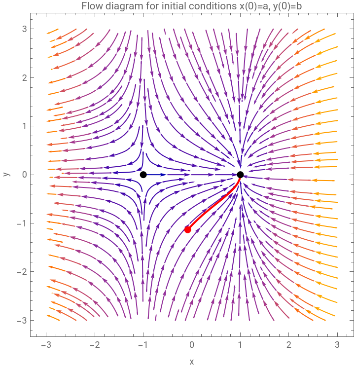
The diagram shows the x-nullclines and y-nullclines. The two equilibrium points, (-1, 0) and (1, 0), are indicated with black points. Two solutions with different initial conditions have been plotted. It can be clearly observed that the equilibrium point on the left is a saddle point, while the one on the right is an attracting node.
Below are the flow diagrams of the linearized systems around the different fixed points. In these, two solution curves have been drawn, showing that the flow behavior is consistent with that of the global system.
Below are the flow diagrams of the linearized systems around the different fixed points. In these, two solution curves have been drawn, showing that the flow behavior is consistent with that of the global system.
For μ=0
For this value of the parameter, the determinant is zero, indicating that the system is degenerate and, therefore, there exist infinitely many fixed points along a line.
When μ = 0 there is a single equilibrium point corresponding to the intersection of the nullclines:
For this value of the parameter, the determinant is zero, indicating that the system is degenerate and, therefore, there exist infinitely many fixed points along a line.
When μ = 0 there is a single equilibrium point corresponding to the intersection of the nullclines:
where the saddle point and the node merge.
The Jacobian matrix for the point (0,0) is:
The Jacobian matrix for the point (0,0) is:
and their corresponding eigenvalues are:
In the figure, the x-nullcline and y-nullcline are represented, and their intersection corresponds to the fixed point (0, 0).
Since the fixed point is non-hyperbolic, an attempt has been made to find a Lyapunov function to provide information about the stability of the point; however, the sign of its derivative could not be determined.
Since the fixed point is non-hyperbolic, an attempt has been made to find a Lyapunov function to provide information about the stability of the point; however, the sign of its derivative could not be determined.
For μ < 0
For μ < 0
In this case, no equilibrium points exist; however, the flow diagram provides valuable qualitative information about the system's behavior.
A region near the origin (0,0) is referred to as a "ghost" or a bottleneck. When the parameter value μ is very small (less than 1), it can be observed that the flow and the trajectories of the solution curves slow down significantly as they pass through this region, as if the fixed point were still present.
In the phase diagram for μ = 0, the solutions reach the horizontal axis. In the case of μ < 0, as the trajectories approach the origin, they decelerate but then deviate to the left, remaining parallel to the horizontal axis without actually touching it.
It is also possible to estimate the approximate time required for a trajectory to cross the ghost region.
Saddle-Node Bifurcation with Invariant Circle
Saddle-Node Bifurcation with Invariant Circle
The saddle-node bifurcation on an invariant circle occurs in nonlinear dynamical systems when a change in a parameter causes the simultaneous appearance or disappearance of equilibrium points of node and saddle type in an invariant circle or limit cycle. This invariant circle is a closed orbit that separates regions of phase space with qualitatively different behaviors. When a critical parameter value is crossed, the node and saddle points emerge on or are annihilated along it. This type of bifurcation is key to understanding transitions between periodic orbits and heteroclinic trajectories in two-dimensional systems.
First of all, we are going to show an example of a two-dimensional system in polar coordinates that exhibits a limit cycle [5].
Note: In this type of system with invariant circles, polar coordinates are usually used because they make it easier to work with limit cycles and interpret them.
First of all, we are going to show an example of a two-dimensional system in polar coordinates that exhibits a limit cycle [5].
Note: In this type of system with invariant circles, polar coordinates are usually used because they make it easier to work with limit cycles and interpret them.
Since the angular equation is constant, it is possible to focus on the radial equation in a one-dimensional system:
Example of the Saddle-Node Bifurcation on an invariant circle or limit cycle
Example of the Saddle-Node Bifurcation on an invariant circle or limit cycle
An example [3] of the Saddle-Node bifurcation on an invariant circle or limit cycle is now presented. This type of bifurcation is commonly referred as a ’Saddle-Node Infinite Period Bifurcation on a Cycle,’ or SNIPER.
It can be observed that the curve does not cross the horizontal axis. Therefore, there are no equilibrium points. From the example of the invariant circle, it is known that the phase diagram has a limit cycle with unit radius and center at (0,0).
It is worth highlighting a behavior that occurs in limit cycles. In some regions of this circle, the flow can be observed to be slow, while in others the flow is faster. This is related to the graph shown. The local minimum at π/2 corresponds to slow flow, whereas at the local maximum 3π/2 the flow is fast. In the flow diagram, this translates onto the unit circle in polar coordinates, at the “north pole” θ = π/2 the flow is slow, while at the “south pole” θ = 3π/2 the flow is fast.
Now we plot the graph for μ = 1:
An intersection between the curve and the horizontal axis is obtained at θ = π/2, which corresponds to a saddle point. This makes sense, since the flow slows down in that region, and at the point θ = π/2 the bifurcation value has appeared. At the saddle point, the flow will pass through it, but in the rest of the invariant circle, the flow will be faster.
The following case occurs when the curve is no longer tangent to the axis and an intersection appears, giving rise to two fixed points: a node and a saddle point, 0<μ<1.
Now, the graph is plotted for μ = 0.5:
The following case occurs when the curve is no longer tangent to the axis and an intersection appears, giving rise to two fixed points: a node and a saddle point, 0<μ<1.
Now, the graph is plotted for μ = 0.5:
An intersection is obtained between the curve and the horizontal axis at two points, where there will be an attractor on the left and a repulsor on the right.
In the phase diagram, these two points will appear on the invariant circle and originate from the north pole at θ = π/2, where the attractor will gradually move to the right along the circle. In the 2D system, the unstable point is a saddle point that will move to the left.
For the node and the saddle, since polar coordinates are being used, the radial line originating at (0,0) and passing through the two points (all points in space with the same angle as the stable point, but with different radii) causes the flow passing through them to go directly to the point. These two lines are the stable manifolds of the two points.
The phase diagrams are shown below.
For μ=2
For μ=2
For μ = 1
For μ = 1
For μ = 0.5
For μ = 0.5
Hopf Bifurcations
Hopf Bifurcations
Hopf or Andronov–Hopf bifurcations are considered as the appearance or disappearance of a periodic orbit through a local change in the stability properties (parameter) of an equilibrium point. In other words, it is a critical point at which the stability of a system changes and a periodic solution emerges.
It can be verified whether the bifurcation is of Hopf type or not by examining the imaginary components of the dominant eigenvalues whose real parts are at a critical value (zero). If there are nonzero imaginary components, it must be a Hopf bifurcation. The periodic orbits of the system that originate near the bifurcation point are known as limit cycles, and the stability of the periodic orbit is determined by the sign of the first Lyapunov coefficient.
Using the trace–determinant plane, when studying the stability of different equilibrium points, one can draw the curve of parameter values and observe how the behavior of the system’s flow changes. Hopf bifurcations occur when the system transitions from having complex eigenvalues with negative real parts (or zero) to positive ones, and vice versa. If the parameter curve is plotted on the trace–determinant plane and crosses the positive ordinate axis, a Hopf bifurcation will occur.
The following theorem (whose proof can be found in [4] from pages 13 to 27) allows transforming any system with a Hopf bifurcation into another that is topologically equivalent.
Let there be a dynamical system that exhibits Hopf bifurcations. Then this system is topologically equivale to the following system:
This form is known as the topological normal form.
- Hopf bifurcation
- Hopf bifurcation
Performing the change to polar coordinates, we obtain:
Therefore, the resulting system is:
A Manipulate function is used to modify the parameters μ and λ of the general Hopf equations in order to visualize them.
Care must be taken not to assign values of μ and λ that are too different, since the system becomes stiff and does not provide a drawable solution.
Care must be taken not to assign values of μ and λ that are too different, since the system becomes stiff and does not provide a drawable solution.
Neuronal Model with Hopf Bifurcation
Neuronal Model with Hopf Bifurcation
In this section, a neuronal model will be studied, and the parameter values that produce a Hopf bifurcation will be sought, since such a bifurcation generates a periodic voltage in the artificial neuron.
The study begins with the initial neuronal model from the article “Iontronic Nanopore Model for Artificial Neurons: The Requisites of Spiking” by Juan Bisquert [1].
The study begins with the initial neuronal model from the article “Iontronic Nanopore Model for Artificial Neurons: The Requisites of Spiking” by Juan Bisquert [1].
In this way, it is clearly seen that there are two nullclines:
- p-nullcline:
- p-nullcline:
From the previous system,
From the model, the expression for g(u,p) is:
Then the p-nullcline is:
Solving for the variable p:
Solving the expression for K(u), we obtain the final expression:
- u nullcline:
- u nullcline:
From the previous system,
Then, the nullcline is:
Solving for the variable u:
Solving for the current 𝐼:
Substituting with the expression for the p-nullcline:
Using the expression for the p-nullcline:
The equilibrium points will be those where the system is in a steady state.
The curve 𝐼(𝑢) can be represented, over which the bifurcation values of the parameter 𝐼 will be sought.
In the theoretical section where the Hopf bifurcation is explained, it is mentioned that the bifurcation value is obtained when the trace of the matrix associated with the system of ordinary differentia equations becomes zero, and its corresponding eigenvalues have zero real part and nonzero imaginary part.
The linearized system will be:
Where:
where:
The expression for the determinant is:
where:
Therefore, the equilibrium points are found where the trace is zero and the determinant is positive.
Now an example will be carried out to find the value of the intensity that makes the neuron’s stimulus periodic. For this, the parameter values from Figure 2(d) of [1] will be used. To obtain the bifurcation value, the trace-determinant theorem will be used.
Next, the system functions are defined along with the trace of the linearized system matrix.
Conclusions
Conclusions
Through this study, a deeper understanding of two-dimensional systems of partial differential equations has been achieved. The research has explored, through independent analysis, the field of bifurcations in dynamical systems, with particular emphasis on those arising in neuronal models. Specifically, saddle–node bifurcations, saddle–node bifurcations on an invariant circle, and Hopf bifurcations have been investigated.
The importance of bifurcations—especially Hopf bifurcations—has been highlighted due to their ability to model neuronal behavior and information transmission processes. These bifurcations provide deeper insight into the underlying dynamics of the electrical impulses that characterize nervous system activity. In particular, Hopf bifurcations are essential for describing transitions between oscillatory and non-oscillatory regimes, phenomena that are fundamental to the propagation of neural signals. This enables a more accurate representation of the complex behavior of neuronal systems.
Through mathematical modeling it becomes possible to simulate more realistic neural networks and predict neuronal responses to different stimuli with higher accuracy. Furthermore, the potential of these mathematical techniques opens the path toward the development of artificial neural models that may, in the future, emulate the functionality of the human brain. Such approaches hold significant promise for advancing both neuroscience research and neuroinformatics technology.
In summary, this work reaffirms the central role of mathematics as an essential tool for understanding the fundamental mechanisms of the brain and for guiding the development of functional artificial neural models.
Acknowledgements
Acknowledgements
We want to thank our professors Alicia Cordero Barbero and Juan Ramón Torregrosa Sánchez for their help and showing us the world of bifurcations in PDE systems. We also want to thank the Wolfram Mathematica team for giving us the opportunity to share our work with the world.
References
References
[1] Bisquert, J ., Iontronic Nanopore Model for Artificial Neurons : The Requisites of Spiking The Journal of Physical Chemistry Letters, 14 (40) : 9027–9033, 2023.
[2] Hopper, A . J ., Beswick - Jones, H ., Brown, A . M ., A color - coded graphical guide to the Hodgkin and Huxley papers Advances in Physiology Education, 46 (4): 580–592, 2022.
[3] Koon, W . S ., Lo, M . W ., Marsden, J . E ., Ross, S . D ., Dynamical Systems, the Three Body Problem and Space Mission Design . Marsden Books, 2022.
[4] Garcia Soria, A ., Atravesando lentamente una bifurcacion de Hopf . Oviedo, Universidad de Oviedo, 2023.
[5] Bramburger, J . J ., Data - Driven Methods for Dynamic Systems . Philadelphia, Society for In dustrial and Applied Mathematics, 2024.
[6] L . Perko ., Differential equations and dynamical systems . Springer, 2001
CITE THIS NOTEBOOK
CITE THIS NOTEBOOK
Introduction to bifurcations in two-dimensional systems of differential equations in artificial neuron models
by Damián Oussa Vañó Fernández, Xuan Liu & Antonio Sineiro Abal
Wolfram Community, STAFF PICKS, November 5, 2025
https://community.wolfram.com/groups/-/m/t/3570974
by Damián Oussa Vañó Fernández, Xuan Liu & Antonio Sineiro Abal
Wolfram Community, STAFF PICKS, November 5, 2025
https://community.wolfram.com/groups/-/m/t/3570974