Wolfram Computational Research Club at SUNY Korea
Seohyun Cho
Stony Brook University, Korea
Stock prices are notoriously difficult to predict. While the Efficient Market Hypothesis suggests that future price movements should be largely unpredictable, momentum investing has remained one of the most persistent anomalies in financial markets. This essay investigates whether momentum-related features can improve stock direction prediction beyond a naive always-up benchmark. Using monthly data from four large-cap U.S. technology stocks (AAPL, MSFT, NVDA, and AMZN) between 2015 and 2024, the analysis constructs four momentum-based features: one-month return, three-month return, six-month return, and rolling volatility. Logistic regression and random forest classifiers are then trained to predict whether the next month’s return will be positive or negative.
The models’ predictive performance is evaluated against two benchmarks: random guessing and a naive strategy that always predicts positive returns. Results show that while the classifiers occasionally perform slightly above random chance, they generally fail to outperform the always-up benchmark consistently. Random forest sometimes matches the benchmark, but neither model clearly exceeds it across the four stocks examined. These findings suggest that simple momentum and volatility features contain limited predictive information for monthly stock-direction forecasting, highlighting both the difficulty of financial prediction and the strong upward drift present in large-cap equity markets during the sample period.
The models’ predictive performance is evaluated against two benchmarks: random guessing and a naive strategy that always predicts positive returns. Results show that while the classifiers occasionally perform slightly above random chance, they generally fail to outperform the always-up benchmark consistently. Random forest sometimes matches the benchmark, but neither model clearly exceeds it across the four stocks examined. These findings suggest that simple momentum and volatility features contain limited predictive information for monthly stock-direction forecasting, highlighting both the difficulty of financial prediction and the strong upward drift present in large-cap equity markets during the sample period.
1. Introduction
Momentum investing is based on a simple idea: stocks that performed well recently may continue to perform well in the near future. This phenomenon has been widely documented in financial markets and remains one of the most studied market anomalies (Jegadeesh and Titman, 1993). Traditional momentum strategies typically rely on a single signal, such as the cumulative return over the previous six months, to rank stocks and guide investment decisions.
However, financial markets are noisy, and any single momentum signal may fail to capture broader market behavior. This raises an important question: can combining multiple momentum-related features improve predictive performance? Instead of using only one past return measure, this essay considers four features: the one-month return, three-month return, six-month return, and recent rolling volatility. A machine learning classifier is then trained to predict whether the next month’s stock return will be positive or negative.
To evaluate whether these features contain meaningful predictive information, the classifier is compared against a deliberately simple benchmark: a strategy that always predicts positive returns. Because equity markets tend to rise more often than they fall, this naive benchmark can achieve approximately 55–60% directional accuracy without using any financial indicators or machine learning methods. Comparing model performance against this benchmark provides a practical test of whether momentum-related features offer predictive value beyond the general upward drift of stock markets.
2. Data and Log Return Computation
Monthly closing prices for four large-cap U.S. technology stocks (AAPL, MSFT, NVDA, and AMZN) are collected from January 2015 through December 2024. This produces approximately 120 monthly price observations and 119 monthly return observations for each stock. Large-cap technology companies are selected because they are highly liquid, widely traded, and strongly associated with momentum-driven market behavior during this period.
Rather than using raw stock prices directly, the analysis computes monthly log returns as the first difference of logarithmic prices:
r
t
P
t
P
t-1
where P_t represents the monthly closing price at time t. Log returns are commonly used in quantitative finance because they are additive across time, making multi-period momentum calculations more consistent. They also place stocks with very different price levels on a comparable scale.
The resulting return series captures the month-to-month fluctuations of each stock, including both sharp declines and strong rallies during periods such as the COVID-19 market crash and the subsequent technology-driven recovery. These return series form the foundation for all subsequent feature construction and machine learning classification models used throughout the essay.
2.1 Data Retrieval and Log Return Computation
2.1 Data Retrieval and Log Return Computation
The following code retrieves monthly stock price data and computes log returns for each stock.
Define the stock tickers used in the analysis.
In[]:=
stocks={"AAPL","MSFT","NVDA","AMZN"}
Out[]=
{AAPL,MSFT,NVDA,AMZN}
Retrieve monthly stock price data for each stock.
In[]:=
rawData=Association[Table[stock->FinancialData[stock,{{2015,1,1},{2024,12,31},"Month"}],{stock,stocks}]];
Extract the numerical monthly closing prices.
In[]:=
prices=Association[Table[stock->QuantityMagnitude[rawData[stock]["Values"]],{stock,stocks}]];
Compute monthly log returns.
In[]:=
logReturns=Association[Table[stock->Differences[Log[prices[stock]]],{stock,stocks}]];
Check the number of return observations.
In[]:=
Map[Length,logReturns]
Out[]=
AAPL119,MSFT119,NVDA119,AMZN119
Construct the corresponding date axis for the return series.
In[]:=
dates=Association[Table[stock->Rest[rawData[stock]["Dates"]],{stock,stocks}]];
Each stock produces 119 monthly return observations, which is expected because returns are calculated from changes between consecutive monthly prices. The aligned return series allows the same feature construction and classification procedure to be applied consistently across all four stocks.
Plot AAPL monthly log returns to visualize the behavior of the return series before constructing momentum features and training classification models.
In[]:=
DateListPlot[Transpose[{dates["AAPL"],logReturns["AAPL"]}],PlotLabel->"AAPL Monthly Log Returns (2015–2024)",AxesLabel->{"Date","Log Return"},Filling->Axis,PlotTheme->"Scientific",ImageSize->Large]
Out[]=
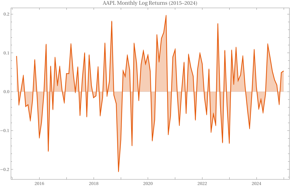
AAPL monthly log returns are plotted as an example of the return series used throughout the analysis. The series fluctuates around zero, with occasional large positive and negative movements. Notable spikes appear during periods such as the COVID-19 market disruption in early 2020 and the strong technology-sector rally in 2023. These fluctuations illustrate why predicting monthly stock direction is difficult: returns are noisy, highly variable, and exhibit periods of volatility clustering rather than constant variance over time.
3. Momentum Feature Construction
Momentum investing is based on a simple intuition: a stock that has been rising tends to keep rising, at least for a while. Think of it like a moving train, it takes time to slow down or reverse. The question this essay asks is whether that “train speed”, measured by recent returns and volatility, is enough information to predict which direction the train will go next month.
Traditional momentum strategies often rely on a single signal: the past six-month return. This essay expands on that idea by constructing four features for each stock at each month. Each feature is lagged by one period to prevent data leakage, meaning that the features used to predict month t+1 are computed only from information available by the end of month t.
The four features are: • ret1: one-month log return • ret3: three-month cumulative log return • ret6: six-month cumulative log return • vol6: rolling six-month standard deviation of returns
The prediction target is the sign of next month’s log return: +1 if the return is positive and -1 if the return is negative. This converts the task from return forecasting into binary classification, making it directly comparable to a simple directional benchmark.
3.1 Feature Engineering
3.1 Feature Engineering
Define a function that constructs momentum features and next-month direction labels from a monthly return series.
In[]:=
buildFeatures[ret_List]:=Module[{n,ret1,ret3,ret6,vol6,label},n=Length[ret];ret1=ret[[7;;n-1]];ret3=Table[Total[ret[[i-2;;i]]],{i,7,n-1}];ret6=Table[Total[ret[[i-5;;i]]],{i,7,n-1}];vol6=Table[StandardDeviation[ret[[i-5;;i]]],{i,7,n-1}];label=Sign[ret[[8;;n]]];{Transpose[{ret1,ret3,ret6,vol6}],label}];
Build the feature matrix and label vector for AAPL.
In[]:=
{features,labels}=buildFeatures[logReturns["AAPL"]];
Check the dimensions of the feature matrix.
In[]:=
Dimensions[features]
Out[]=
{112,4}
Check the number of direction labels.
In[]:=
Length[labels]
Out[]=
112
Count the number of positive and negative return months.
In[]:=
Counts[labels]
Out[]=
-147,165
The feature-construction function creates a feature matrix and label vector from AAPL’s monthly return series. The result contains 112 labeled observations with four features each. Among these observations, 65 months are positive and 47 months are negative, showing that the sample has an upward bias but still includes a substantial number of down months.
3.2 Scatter Plot: 3-Month Return vs. Next-Month Direction
3.2 Scatter Plot: 3-Month Return vs. Next-Month Direction
To visually inspect whether momentum separates future up and down months, this plot compares AAPL’s three-month cumulative return with the following month’s return. If momentum were a strong directional predictor, positive and negative months would form clearly separated clusters.
Identify months with positive and negative next-month returns.
In[]:=
upIdx=Flatten[Position[labels,1]];downIdx=Flatten[Position[labels,-1]];nextRet=logReturns["AAPL"][[8;;Length[logReturns["AAPL"]]]];
Plot three-month momentum against next-month return.
In[]:=
ListPlot[{Transpose[{features[[upIdx,2]],nextRet[[upIdx]]}],Transpose[{features[[downIdx,2]],nextRet[[downIdx]]}]},PlotLabel->"3-Month Momentum vs. Next-Month Return (AAPL)",AxesLabel->{"3-Month Return","Next-Month Return"},PlotLegends->{"Up (+1)","Down (-1)"},PlotTheme->"Scientific",PlotStyle->{Blue,Orange},ImageSize->Large]
Out[]=
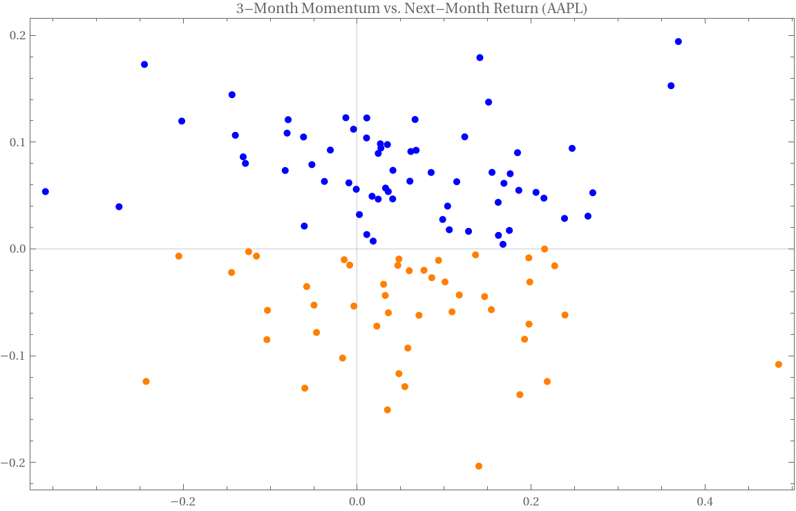


The scatter plot shows substantial overlap between positive and negative next-month returns across the full range of three-month momentum values. Although some high-momentum months are followed by positive returns, there is no clean separation between the two groups. This suggests that three-month momentum may contain limited directional information, but it does not produce a clear decision boundary for predicting next-month stock direction.
3.3 Feature Correlation Matrix
3.3 Feature Correlation Matrix
Before training the classifier, it is useful to examine how the four features relate to each other. The correlation matrix shows whether the momentum and volatility variables capture distinct information or overlap with each other.
Compute the correlation matrix for the four features.
Create tick labels for the correlation matrix plot.
Visualize the feature correlation matrix.
Display the numerical correlation matrix.
Compute the Correlation Matrix
The correlation matrix shows that the return-based momentum features are positively correlated. In particular, ret3 and ret6 have the strongest correlation because the six-month return window contains much of the information from the three-month window. By contrast, vol6 has weak correlations with ret1, ret3, and ret6, suggesting that recent volatility captures a different aspect of the data: risk rather than recent performance. This supports including vol6 as a separate feature, while also showing that several momentum variables may contain overlapping information.
4. Machine Learning Classifier
A logistic classifier works like a scorecard. It assigns a weight to each feature (recent return and volatility) and combines them into a single prediction score. If the score crosses a threshold, the model predicts that the stock will move up next month; otherwise, it predicts down. A random forest works differently. Instead of using one linear rule, it builds many decision trees using different subsets of the data and features, then combines their predictions through majority voting. The key difference is flexibility: logistic regression can only form a linear decision boundary, while random forest can model more complex nonlinear relationships.
Two classifiers are trained using logistic regression and random forest. Logistic regression provides a simple linear baseline, while random forest allows for more flexible nonlinear decision boundaries. The dataset is divided into a training set containing the first 80 observations and a test set containing the remaining 32 observations. This out-of-sample evaluation is important because testing on the same data used for training would produce unrealistically optimistic results.
4.1 Training and Prediction
4.1 Training and Prediction
Split the data into training and testing sets.
Display the number of training and test observations.
Train the logistic regression classifier and generate predictions.
Inspect the first ten predicted and actual labels.
The logistic regression classifier is trained on the 80-observation training sample and evaluated on the remaining 32 out-of-sample observations. The first ten predictions are all classified as positive months, while the true labels contain several negative months. This suggests that the model may be learning the overall upward tendency of the stock market rather than identifying reliable month-specific directional signals. Because positive months occur more frequently than negative months in the sample, predicting “up” repeatedly can still produce moderate accuracy even if the model fails to detect meaningful momentum patterns.
5. Evaluation: Can It Beat the Coin Flip?
Before looking at the results, it is important to define what “beating the benchmark” means. A model that randomly guesses up or down would be expected to achieve about 50% accuracy. However, this is not the strongest benchmark in stock direction prediction. Because large-cap U.S. stocks rise more often than they fall, a model that always predicts “up” can often achieve higher accuracy without using any features or machine learning.
This essay therefore compares the classifier against two benchmarks. The first is a coin flip at 50% accuracy, representing random guessing. The second is the naive always-up strategy, which predicts +1 every month. Beating the always-up benchmark is the more meaningful test because it asks whether the momentum features add predictive value beyond the general upward drift of equity markets.
5.1 Accuracy Comparison: AAPL
5.1 Accuracy Comparison: AAPL
Compute the directional accuracy of the logistic classifier and the benchmark models.
Display the accuracy values.
Visualize the directional accuracy comparison.
The logistic classifier achieves 50.0% directional accuracy on the AAPL test set, which is equivalent to coin-flip performance. The naive always-up benchmark achieves 56.25%, meaning that simply predicting a positive return every month performs better than the machine learning model. This result suggests that the four momentum-related features do not provide useful predictive information beyond the overall upward drift present in the test period.
5.2 Confusion Matrix: Why Accuracy Is Misleading
5.2 Confusion Matrix: Why Accuracy Is Misleading
Accuracy alone can hide how a classifier is making its mistakes. A confusion matrix provides a more detailed view by showing how many up and down months are correctly or incorrectly classified.
Create classifier measurements for the AAPL test set.
Display the confusion matrix.
Compute class-specific performance metrics.
The confusion matrix reveals that the classifier’s errors are not random. Instead, they are systematically biased toward predicting upward months. Recall for down months is only 21.4%, meaning the model correctly identifies just 3 of 14 actual down months. In contrast, recall for up months reaches 72.2%, largely because the classifier frequently predicts “up” regardless of the feature values.
This behavior suggests that the model is not extracting a reliable directional signal from the momentum variables. Instead, it is mostly learning the upward drift already present in the stock. A trader using these predictions would remain heavily exposed during market downturns, limiting the practical usefulness of the classifier even when its overall accuracy appears reasonable.
5.3 Multi-Stock Generalization
5.3 Multi-Stock Generalization
To test whether the AAPL result generalizes, the same procedure is repeated for MSFT, NVDA, and AMZN. This checks whether the model’s performance is specific to one stock or consistent across multiple large-cap technology companies.
Train logistic regression and random forest classifiers for each stock, then compare their test accuracy against the always-up benchmark.
Display the accuracy results for all stocks.
Prepare values for the comparison chart.
Visualize logistic regression, random forest, and always-up accuracy across stocks.
Across all four stocks, logistic regression fails to outperform the always-up benchmark. For AAPL, MSFT, NVDA, and AMZN, the logistic classifier either ties or falls below the naive strategy. Random forest performs slightly better in some cases, but it also fails to clearly beat the always-up benchmark. For NVDA, for example, the always-up benchmark reaches 68.75% because of the stock’s strong upward trend, while logistic regression reaches 65.63% and random forest only matches the benchmark.
This pattern suggests that the classifiers mostly learn the general upward bias of large-cap technology stocks rather than extracting a meaningful directional signal from the momentum features. The inclusion of volatility (vol6) also does not materially improve prediction accuracy, suggesting that recent volatility alone is insufficient to separate future up and down months in this dataset.
5.4 Overall Evaluation Summary
5.4 Overall Evaluation Summary
Overall, the evaluation shows that the machine learning models do not meaningfully improve momentum-based directional prediction. Logistic regression performs at coin-flip level for AAPL and fails to beat the always-up benchmark across all four stocks. Random forest performs slightly better in some cases, but it only matches the naive benchmark rather than clearly exceeding it. Therefore, these results suggest that the selected momentum and volatility features are not strong enough to overcome the simple upward bias already present in large-cap technology stocks.
6. Conclusion
This essay asked whether momentum-related features can predict the direction of next-month stock returns better than a naive always-up benchmark. Two classifiers were tested: logistic regression and random forest. For AAPL over the 2015–2024 period, logistic regression achieved 50.0% directional accuracy, falling short of the always-up benchmark at 56.25%. Random forest matched the always-up benchmark exactly at 56.25%, but did not exceed it. Because the test set contains only 32 observations, these results should be interpreted as exploratory rather than definitive.
The same general pattern appears across all four stocks. For MSFT, logistic regression, random forest, and always-up all achieve 53.1% accuracy. For NVDA, random forest matches the always-up benchmark at 68.75%, while logistic regression reaches 65.63%. For AMZN, random forest again matches always-up at 62.5%, while logistic regression reaches 56.25%. In no case does either classifier clearly outperform the naive benchmark.
These findings are informative because they show the difference between beating random guessing and beating a meaningful financial benchmark. Both machine learning models and the naive benchmark can perform above the 50% coin-flip baseline, reflecting the upward bias of equities during the sample period. However, the momentum and volatility features used in this essay do not provide enough additional information to improve directional prediction beyond that upward drift. In particular, the volatility feature (vol6) contributes little additional predictive power beyond the return-based momentum variables, suggesting that recent market risk does not translate cleanly into next-month directional forecasting ability. This result is broadly consistent with the Efficient Market Hypothesis (Fama, 1970), which suggests that simple and publicly observable market patterns may be difficult to exploit consistently.
At the same time, these findings should not be interpreted as evidence against momentum investing in general. This essay focuses on directional prediction for individual large-cap technology stocks rather than cross-sectional momentum portfolios, which are typically constructed differently in academic finance research. In other words, failing to predict whether one stock will rise next month is not the same as disproving momentum as a portfolio strategy.
Future work could apply walk-forward validation instead of a single train-test split, expand the stock universe beyond large-cap technology firms, and evaluate models using portfolio-level metrics such as Sharpe ratio and maximum drawdown rather than directional accuracy alone.
References
◼
Fama, E. F. (1970). Efficient capital markets: A review of theory and empirical work. The Journal of Finance, 25(2), 383–417.
◼
Jegadeesh, N., and Titman, S. (1993). Returns to buying winners and selling losers: Implications for stock market efficiency. The Journal of Finance, 48(1), 65–91.
◼
Wolfram Research (2024). Wolfram Language and System Documentation Center. Classify. Wolfram Research, Inc.