Link Between Autoregressive and Ornstein-Uhlenbeck Processes
Link Between Autoregressive and Ornstein-Uhlenbeck Processes
Autoregressive time series models and continuous time series models such as the ubiquitous Ornstein-Uhlenbeck (OU) process generally arise in different contexts. While the AR process is a staple of traditional time series modeling, the OU process is a widely used stochastic process in various fields, including finance, physics, and biology.
Often the connection between the two processes goes unremarked upon. In fact, the discrete-time AR model converges to the continuous-time OU process under certain conditions.
Often the connection between the two processes goes unremarked upon. In fact, the discrete-time AR model converges to the continuous-time OU process under certain conditions.
The discrete - time AR model can be written as :
X
t+1
ϕX
t
ϵ
t
where is the time series at time t, ϕ is the autoregressive parameter and is the white noise error term with mean zero and variance .
X
t
ϵ
t
2
σ
The continuous - time OU process is defined as :
dX
t
X
t
σdW
t
where is the process at time , is the rate of mean reversion, μ is the long term mean, σ is the volatility, t is an infinitesimally small time interval and s a Wiener process (Brownian motion), representing the stochastic component of the process.
X
t
t
θ
W
t
To demonstrate the correspondence between the two models, we need to show that under certain conditions, the AR model converges to the OU process as the time interval approaches zero.
To derive the connection, we start by taking the limit as the time interval Δt approaches zero, making the AR model a continuous - time process. The noise term will converge to , the Wiener process, under specific conditions.
ϵ
t
W
t
The convergence is ensured if the following conditions hold :
◼
The AR parameter ϕ should be negative and the absolute value of ϕ should be less than 1 to ensure stability.
◼
The variance of the noise term should be related to
σ and Δt.
ϵ
t
σ and Δt.
◼
The mean of should be zero, which is typical in many AR models .
ϵ
t
By taking the limit as Δt approaches zero, the discrete - time AR model converges to the continuous - time OU process :
lim
Δt->0
X
t+1
X
t
Δt
X
t
dW
t
dt
We then equate the terms from the AR model and the OU process to establish the connection between ϕ and θ, and relate the variance of to σ and Δt.
ϵ
t
Step1:RewritethediscreteARmodelusing:
ΔX
t
ΔX
t
X
t+1
X
t
X
t
ϵ
t
ϕX
t
X
t
ϵ
t
Step 2 : Divide by Δt :
ΔX
t
Δt
(ϕ-1)+
X
t
ϵ
t
Δt
Step 3 : Take the limit as Δt approaches zero:
lim
Δt0
ΔX
t
Δt
lim
Δt0
(ϕ-1)
X
t
Δt
lim
Δt0
ϵ
t
Δt
Step 4 : Recognize that is equivalent to σ in the continuous - time OU process .
lim
Δt->0
ϵ
t
Δt
W
t
Step 5 : Take the first limit:
lim
Δt0
(ϕ-1)
X
t
Δt
lim
Δt0
X
t
Δt
Step 6 : Recognize that is equivalent to in the continuous-time OU process.
lim
Δt0
ΔX
t
Δt
X
t
t
Step 7: Rewrite the limit:
lim
Δt0
ΔX
t
Δt
X
t
t
dW
t
dt
Step 8 : Equate the continuous - time OU process and the AR model:
X
t
t
θ(μ-)
X
t
(ϕ-1)
This shows that as Δt approaches zero, the discrete AR model converges to the continuous - time OU process. The correspondence between the two is established, and we find that ϕ and θ are related by:
θ=
2
σ
ϕ-1
Another, simpler approach is to discretize the OU process:
X
Δt+t
X
t
X
t
Δt
ϵ
t
By comparing the two, we can relate the parameters :
ϕ = 1 - θ tμ = 0 (for simplicity) = σ
σ
AR
Δt
Illustration
Illustration
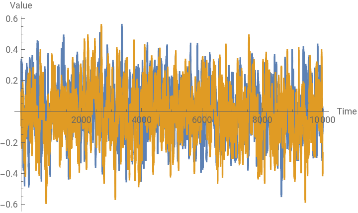
Let' s simulate paths for both processes using the following parameters :
In[]:=
(*Defineparameters*)phi=0.95;sigmaAR=0.05;dt=0.01;theta=(1-phi)/dt;sigmaOU=sigmaAR/Sqrt[dt];mu=0;T=100;steps=Round[T/dt];(*SimulateAR(1)Process*)arPath=NestList[phi#+sigmaARRandomReal[NormalDistribution[0,1]]&,0,steps];(*DiscretizeandSimulateOUProcess*)ouPath=NestList[#+theta(mu-#)dt+sigmaOUSqrt[dt]RandomReal[NormalDistribution[0,1]]&,0,steps];(*Plotthepaths*)ListLinePlot[{arPath,ouPath},PlotLegends->{"AR(1)","OU"},AxesLabel->{"Time","Value"}]
Out[]=


Cumulative Paths
Cumulative Paths
The equivalence between the discrete AR (1) process and the continuous Ornstein - Uhlenbeck (OU) process is more of a theoretical one, particularly when considering infinitesimally small time steps in the OU process. However, when we discretize the OU process, as we' ve done, the two processes can be made to resemble each other over short intervals . Given the parameters we' re using:
ϕ=0.95=0.05Δt=0.01θ==
σ
AR
1-ϕ
Δt
σ
OU
σ
AR
Δt
Here' s what' s happening :
◼
The AR (1) process is defined by its autoregressive parameter ϕ and the standard deviation of the noise .
σ
AR
◼
The discretized OU process' s parameters are derived to match the AR (1) process over a one - step interval . Specifically, θ is chosen to give a similar autoregressive behavior to ϕ, and is adjusted to match the noise level.
σ
OU
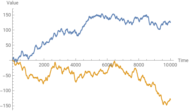
Over short intervals (one - step changes), the two processes should be fairly similar. However, over longer intervals, the cumulative effects of their different dynamics will become evident, especially since the AR (1) lacks the mean - reverting property of the OU process.
For the parameters we’ ve chosen :
For the parameters we’ ve chosen :
◼
The AR (1) process has a strong persistence due to the high ϕ value, meaning it will remember its previous values well.
◼
The OU process will have strong mean - reversion due to the high θ value derived from ϕ and Δt.
The individual paths of the processes will have similar fluctuations around their current values. However, the cumulative paths will differ because of the reasons mentioned above. The AR (1) process will tend to drift, while the OU process will revert to its mean (which is 0 in this case). To get a closer match in the cumulative paths over a longer duration, you would have to adjust the parameters, especially the mean of the OU process μ and its mean - reversion strength θ.
In[]:=
ListLinePlot[{Accumulate@arPath,Accumulate@ouPath},PlotLegends->{"AR(1)","OU"},AxesLabel->{"Time","Value"}]
Out[]=
References
References
◼
Brockwell, P . J ., & Davis, R . A . (1991) . Time Series : Theory and Methods . Springer Science & Business Media. (Chapter 3.5 covers AR processes and their properties).
◼
Box, G . E ., Jenkins, G . M ., Reinsel, G . C ., & Ljung, G . M . (2015). Time Series Analysis : Forecasting and Control. Wiley. (Chapter 5 introduces ARIMA models).
◼
Uhlenbeck, G . E ., & Ornstein, L . S . (1930). On the Theory of the Brownian Motion . Physical Review, 36 (5), 823 - 841. (Original paper on the Ornstein - Uhlenbeck process).
CITE THIS NOTEBOOK
CITE THIS NOTEBOOK
Momentum and mean reversion in discrete and continuous time processes
by Jonathan Kinlay
Wolfram Community, STAFF PICKS, August 2, 2023
https://community.wolfram.com/groups/-/m/t/2981627
by Jonathan Kinlay
Wolfram Community, STAFF PICKS, August 2, 2023
https://community.wolfram.com/groups/-/m/t/2981627