Anisotropic Anderson localisation
By Abhishek Joshi (LNMIIT, Jaipur India),
Sinuhé Perea-Puente (King’s College London, UK)
By Abhishek Joshi (LNMIIT, Jaipur India),
Sinuhé Perea-Puente (King’s College London, UK)
In this proposal we design a simple toy-model for understanding the phenomena of Anderson Localisation in the context of disordered media. By initially introducing the basis theory, then we develop some interactive figures to demonstrate the strong localisation in the tight-binding model. Starting at the unidimensional case, thanks to the size of the system, we will use Exact Diagonalisation approach directly. From there we extend these ideas to higher dimension, to see the role of the internal degrees of the quantum many body system.
An (brief) introduction
An (brief) introduction
In his celebrated paper [1], Philip W. Anderson demonstrate the existence of strong localisation phenomena in a quantum system with a large amount of disorder. This eluded diffusion process, was thanks to a very particular cocktail of ingredients that imply some extraordinary corollaries. Emergent theory and mesoscopic structures arise later in the 80s thanks to this idea of disorder as a ally, rather than classic adversary of symmetry. The classical example is thinking about water and ice. While the solid presents a crystalline structure that allow certain discrete invariant transformation (being an hexagonal ring structure we can easily identify with the Dihedral group ), the liquid isotropic molecule distribution allow to have a continuous rotation symmetry. Also, like the forbidden band crossing for low dimensionality in Condensed Matter Physics, properties like metal-insulator transition heavily rely on the characteristic of the system.
In particular, it has been proposed that for any dimension d, localisation of the states is possible when the disorder is strong enough.For the simplest case, d=1, it can be analytically derived that the localisation appears for any small disorder. In the bi-dimensional case, there is currently no exact solution, but it can be numerically approximated via Renormalisation Group [2] analysis for different scales. Many recent lab experiments [3] double-check this techniques. Finally, for higher dimensions, the delocalisation critical strength for the disorder is dependent on the energy of the eigenstates.
D
12
In particular, it has been proposed that for any dimension d, localisation of the states is possible when the disorder is strong enough.For the simplest case, d=1, it can be analytically derived that the localisation appears for any small disorder. In the bi-dimensional case, there is currently no exact solution, but it can be numerically approximated via Renormalisation Group [2] analysis for different scales. Many recent lab experiments [3] double-check this techniques. Finally, for higher dimensions, the delocalisation critical strength for the disorder is dependent on the energy of the eigenstates.
Basic numerical tools and results
Basic numerical tools and results
To properly look at this phenomenon in a lattice, we need to carefully study three different aspects. First of all we can identify (de)-localised states by its energy configuration. The characteristic spectra will correspond to discrete or continuous distributions.We will also need to analyse the Hamiltonian structure, with the corresponding spectral decomposition, via exact diagonalisation methods. And finally, we will study the time-dependent evolution of the Cauchy problem, via the return probability of the electrons. If it is fixed in time and not propagates and therefore we will have an Anderson localisation.
Traditionally, the approach is performed by the following random walk toy-model with the rule "in one dimension, a particle has a probability p to go left, and 1-p to go right”, similar to Einstein’s Brownian motion approximation (then we are going to assume p=1/2 by symmetry).
From classical statistics, this Bernoulli distribution sampling could be described by a Gaussian (normal) distribution thanks to Central Limit Theorem, as we can see below. We can easily calculate the different probabilities of the particle in the lattice [, ] to be at a certain position =k while having steps, with all ∈Z:
x
min
x
max
x
end
s
x
i
p(xk)
s |
k |
s-k
k
p
In[]:=
Manipulate[ListPlot[Table[Binomial[s,k]*(p^k)*(1-p)^(s-k),{k,0,s}], Filling->Axis],Style["Random Walk Distribution [left probability,steps]="Dynamic[p]Dynamic[s], 12, Bold],{{s,17,"Number step"},0,100,1,ImageSize -> Medium,ControlPlacement->Top},{{p,0.6,"Left probab"},0.1,0.9,ImageSize -> Medium},ControlPlacement->Top]
Out[]=


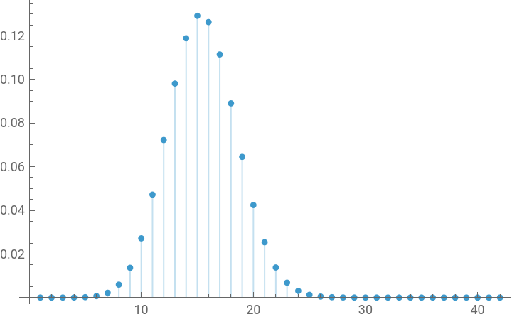
With the peak displaced in accordance with the anisotropy. From here, we can study the self-return probability,corresponding to the situation in which the electron return into its original position later a given number of steps, that it will be given by:
P(xs/2)
s |
s/2 |
s/2
s/2
p
(1-p)
2s |
s |
s
s
p
It is easy to compute its value, thanks to the appearance of central binominal coefficient, related to the Catalan numbers and where we can apply the Stirling formula < n! <and bound this expression, for enough big samples (like in a quantum system):
2πn
n
n
n
e
1/(12n+1)
e
2πn
n
n
n
e
1/(12n+0)
e
Manipulate[Module[{prob},prob=p^n*(1-p)^n;Plot[{prob*Exp[1/(24*n+1)-2/(12*n+1)]*2^(2*n)/Sqrt[Pi*n],prob*Binomial[2*n,n],prob*Exp[1/(24*n)-2/(12*n)]*2^(2*n)/Sqrt[Pi*n]},{n,1,nmax},PlotLegends->{"Higher bound","Exact","Lower bound"}]],Style["Self-return probability left probability="Dynamic[p], 12, Bold],{{p,0.6,"Left probability"},0.1,0.9,ImageSize -> Large,ControlPlacement->Top},{{nmax,2,"Number of steps"},2,30,ImageSize -> Large,ControlPlacement->Top}](*It fits so well that the curves overlap, zoom in to see it*)
Out[]=


It is interesting seeing how the maximum uncertainly correspond to the isotropic case, p=0.5. In any case, from here, it is automatic to compute the correspond expected value of the self-return probability, as the infinite sum
In[]:=
Manipulate[Module[{prob},prob=N[p^n*(1-p)^n,100];Sum[prob*Binomial[2*n,n],{n,1,nmax}]],Style["Self-return, probability="Dynamic[p], 12, Bold],{{p,0.6,"Left probability"},0.3,0.8,ImageSize -> Tiny,ControlPlacement->Top},{{nmax,2,"Number of steps"},2,400,ImageSize -> Tiny,ControlPlacement->Top}]
Out[]=
It is easy to prove that the isotropic case gave a divergent expression as:
〈Self-return〉P(xs/2,p=1/2)=
~∼∞
∞
∑
s=1
∞
∑
s=1
2s |
s |
s
1
2
s
1-
1
2
∞
∑
s=1
2π[2n]
2n
2n
e
2
(2πn)
n
n
e
2s
1
2
1
π
∞
∑
s=1
1
s
Indeed this argument could be easily generalised for higher dimensions d as:
〈d-return〉∼?
1
d/2
π
∞
∑
s=1
1
d/2
s
Where we can see the critic limit in the harmonic sequence, starting with d=2. We can jump into the quantum analogous via another toy-model, the tight binding approximation, discretizing the Schrodinger equation, and where the Hamiltonian can be written (second quantisation) as diagonal and adjacent not trivial positions:
H|s〉〈s|-|s〉〈s+1|-|s+1〉〈s|
n
∑
s=1
ϵ
s
down
g
up
g
corresponding to on-site and hopping terms, that moves the particles to neighbouring site (in principle different).Iin absence of disorder, we obtain a transalationally invariant close system with planes waves as eigenstates(x), with known energy eigenvalues -+cos(). Now we want to compute the effect of the disorder in the system, for what we perform, rather the analytical transfer matrix method, the numerical approach via exact diagonalisation method. The idea is to set values for the hoping terms and assuming that the onsite energy follows an uniform distribution [-W/2,W/2].
Ψ
s
i·
k
s
x
s
e
E
s
up
g
down
g
n
∑
s=1
x
s
ϵ
n
In[]:=
Manipulate[Module[{one,uniform,MM,eVal,eVec},one = ConstantArray[1,m];uniform=RandomVariate[UniformDistribution[{-W/2,W/2}],m+1](* RandomReal[{-w/2,w/2},m]*);MM=gdown*DiagonalMatrix[one,1]+gup*DiagonalMatrix[one,-1]+DiagonalMatrix[uniform];MM〚1〛〚-1〛=MM〚-1〛〚1〛=1;(*M//Dimensions*)eVal=Eigenvalues[MM];eVec=Eigenvectors[MM];(*ListPlot[eVal,PlotRange->Automatic]*)ListPlot[(eVec〚{1,3,5,8}〛)^2,JoinedTrue,PlotLabel->{"Anisotropic Anderson Localisation W=", W},PlotRange{{0,m+1},All}]],{{m,99,"System size" (n)},8,200,1,ImageSize -> Large,ControlPlacement->Top},{{W,1,"Onsite energy (W)"},0,6,ImageSize -> Large,ControlPlacement->Top},{{gup,1,"Up hoping"},0.1,1.9,ImageSize -> Large,ControlPlacement->Top},{{gdown,1,"Down hoping"},0.1,1.9,ImageSize -> Large,ControlPlacement->Top}]
Out[]=
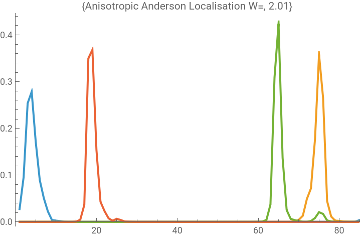
The results show how for W=0, our Hamiltonian have Bloch waves as it’s eigen states. As the disorder is zero , this is just a periodic potential from Bloch theorem.Increasing the disorder (more dispersion of the on-site values), we can see how as we increase the disorder , the waves become more localised.
Further discussion
Further discussion
In this article we have shown Localization in 1-D using Exact Diagonalisation approach. Further work , would be to generalize to higher dimension systems introducing locator expansions and scaling theory.It would be interesting to see ergodicity breaking in many-body localised systems.
Acknowledgement
Acknowledgement
We would like to thank Adiba Shaikh (IIT Bombay, India) for her help in Mathematica essentials for the plots we achieved.
Further references
Further references
[1] Anderson, P. Absence of Diffusion in Certain Random Lattices. Physical Review, 109(5), pp.1492-1505, (1958).
[2] Chenguang G., Xingyue G. , A brief introduction to Anderson Localization, Lecture Massachusetts Institute of Technology (2019).
[3] Lahini, Y. Direct Observation of Anderson Localized Modes and the Effect of Nonlinearity. Photonic Metamaterials: From Random to Periodic (META), The Bahamas (2006).