ABSTRACT (original article): This work explores the rich structure of spherically symmetric time-periodic solutions of the cubic conformal wave equation on . We discover that the families of solutions bifurcating from the eigenmodes of the linearised equation form patterns similar to the ones observed for the cubic wave equation. Alongside the Galerkin approaches, we study them using the new method based on the Padé approximants. To do so, we provide a rigorous perturbative construction of solutions. Due to the conformal symmetry, the solutions presented in this work serve as examples of large time-periodic solutions of the conformally coupled scalar field on the anti-de Sitter background. CITATION (original article): Ficek, F., & Maliborski, M. (2025). Complex structure of time-periodic solutions decoded in Poincaré-Lindstedt series: The cubic conformal wave equation on S3. Physica D: Nonlinear Phenomena, 481. https://doi.org/10.1016/j.physd.2025.134864
3
S
This notebook contains symbolic and numerical computations related to our recent work on the structure of time-periodic solutions in nonlinear wave equations on bounded domains [1–3]. The main focus is the conformally invariant cubic wave equation on the Einstein cylinder [4,5],
2
∂
t
2
∂
x
u
3
(t,x)
2
sin
which arises naturally as a toy model in the study of nonlinear dynamics of asymptotically anti–de Sitter (AdS) spacetimes in General Relativity.
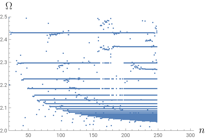
The central theme of this research is that high-order Poincaré–Lindstedt expansions encode information far beyond the small-amplitude regime. While rigorous results [6–9] prove the existence of small-amplitude solutions with frequencies in Cantor-type sets, we show that when combined with Padé resummation the Poincaré–Lindstedt expansion reveals the complex, fractal-like bifurcation structure of time-periodic solutions, extending the description well into the finite-amplitude regime.
This notebook documents the computational procedures behind these results, including perturbative construction, series manipulations, and Padé resummation.
• In Section Code we set up temporal and spatial grids and implement transformations between grid values and trigonometric coefficients (see [10]). Calculations are performed in arbitrary precision arithmetic to control rounding errors, with grid sizes chosen to eliminate aliasing.
• Section Deriving perturbative solution implements the Poincaré–Lindstedt construction following [4]. Solutions bifurcate from the single-mode linear solution
ΩN, (τ,x)cosτ sin(Nx), τΩt
(0)
u
with . (The present code works for even N; the odd case is left as an exercise for interested readers.)
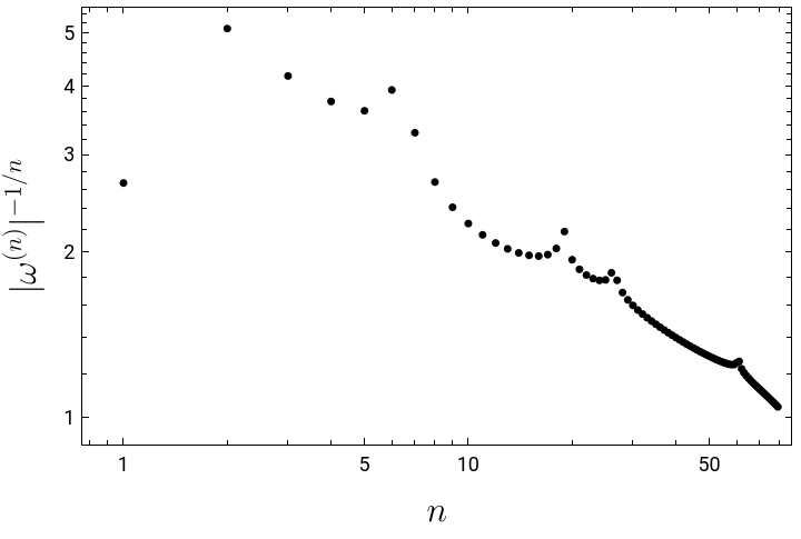
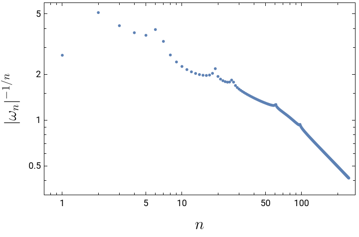
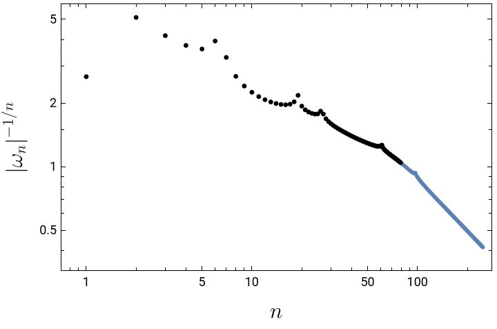
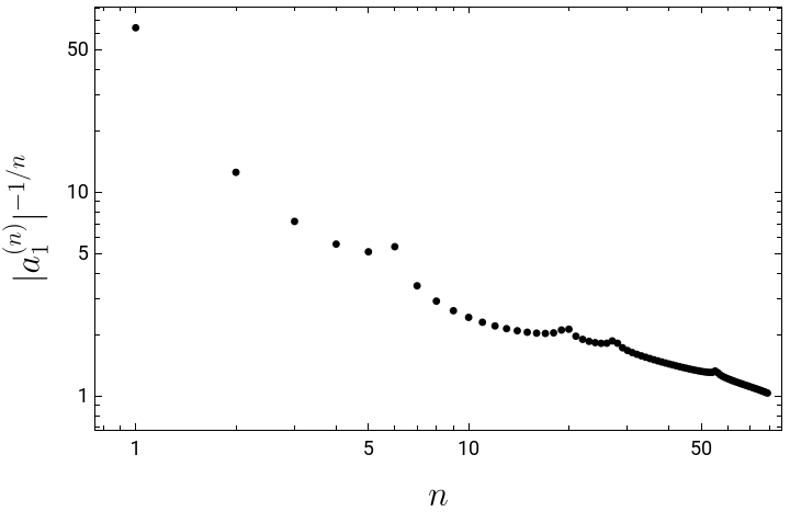
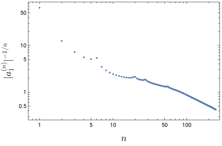
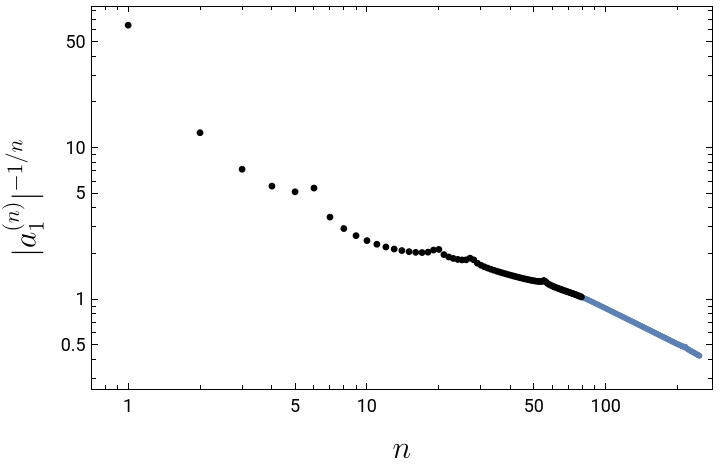
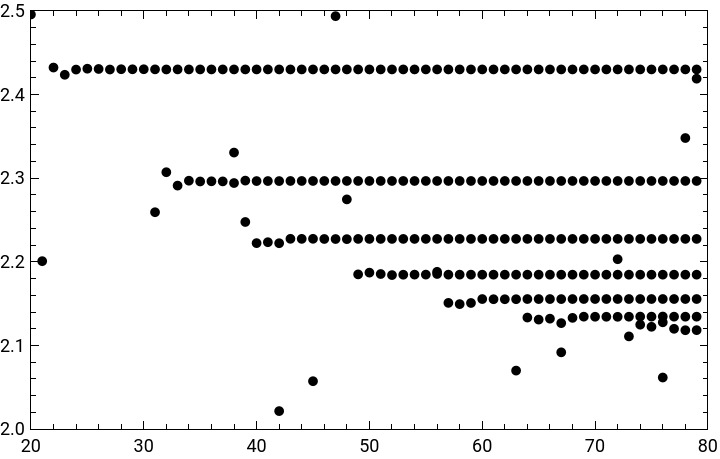
• Section Analysis studies the resulting series. We reproduce Figs. 5 and 7 of [4], showing growth of coefficients (implying zero radius of convergence) and demonstrating that Padé approximants recover global solution features, including the location of bifurcations.
N∈
• Section Analysis studies the resulting series. We reproduce Figs. 5 and 7 of [4], showing growth of coefficients (implying zero radius of convergence) and demonstrating that Padé approximants recover global solution features, including the location of bifurcations.
Practical note: depending on the grid sizes nt and nx, the computations can be memory- and time-intensive. For illustration, we set nt=80 and nx=160, which allows us to reach perturbative order 79. To avoid aliasing and reach the maximal order, one should set nx=N*nt, where N is the mode number of the solution at the lowest order. The main loop over perturbative orders outputs the current order, time and date, and the residual norm of the expansion, which grows with rounding errors. The working precision (prec) can be increased if needed.
Code
Code
General settings
General settings
Additional packages
Needs["MaTeX`"]; (* For generating plot labels *)
To use machine precision use prec=MachinePrecision
prec=128;If[prec==MachinePrecision,$MinPrecision=0;$MaxPrecision=Infinity;,$MinPrecision=prec;$MaxPrecision=prec;];
Temporal grid (cos(t), cos(3 t), cos(5 t), ... )
Temporal grid (cos(t), cos(3 t), cos(5 t), ... )
Spatial grid (sin(2x), sin(4x), ...)
Spatial grid (sin(2x), sin(4x), ...)
Tools
Tools
Deriving perturbative solution
Deriving perturbative solution
Analysis
Analysis
Suppresses precision - related warnings when plotting data and generating Padé approximants. This does not affect the results, but avoids unnecessary (and rather annoying) messages.
Off[SetPrecision::precsm,N::preclg,Solve::preclg,N::precsm];
In[]:=
ord=nmax
Out[]=
79
Reproducing Fig. 5
Reproducing Fig. 5
In[]:=
plot5a=ListLogLogPlotTable,{n,1,ord}//N,FrameLabel->(MaTeX/@{"n","|\\omega^{(n)}|^{-1/n}"}),PlotStyle->Black
-1/n
Abs[ω[n]]
-2
NN
Out[]=
In[]:=
Show
,plot5a
Out[]=
In[]:=
plot5b=ListLogLogPlotTable,{n,1,ord}//N,FrameLabel->(MaTeX/@{"n","|a_{1}^{(n)}|^{-1/n}"}),PlotStyle->Black
-1/n
Abs[a[n][1]]
Out[]=
In[]:=
Show
,plot5b
Out[]=
Generating sums and Padé approximants (see Sec. 4.3)
Generating sums and Padé approximants (see Sec. 4.3)
ω
ω
In[]:=
Clear[ω2sum];ω2sum[ϵ_]=NN^2+Sum[ω[n],{n,1,ord}];
n
ϵ
2
x
Monitor[Do[ω2PadeL[m][x_]=PadeApproximant[ω2sum[]//PowerExpand,{x,0,m}],{m,20,ord}],{"ω",m}]
2
x
a’s
a’s
2
x
Clear[asum];Doasum[(2k+1)][ϵ_]=,{n,k,ord-1}]/.{a[0][1]->1},{k,0,ord};
ϵ
Sum[a[n][(2k+1)]n
(ϵ)
b’s and data for Fig. 7
b’s and data for Fig. 7
In[]:=
Clear[bsum,bPadeL,tabRes];
b
3,8
b
5,12
b
7,16
b
9,20
2
x
Do{j,k}=jk;bsum[j,k][ϵ_]=,{n,0,ord}]/.{b[_][__]->0};Do[bPadeL[m][x_]=PadeApproximant[(bsum[j,k][])//PowerExpand,{x,0,m}],{m,20,ord}];Monitor[tabRes[j,k]=Flatten[Table[DeleteDuplicates[{m,Sqrt[ω2PadeL[m][x]]}/.Solve[Denominator[bPadeL[m][x]]==0,x,Reals,WorkingPrecision200]],{m,20,ord}],1],m];,{jk,{{3,8},{5,12},{7,16},{9,20}}}
ϵ
Sum[b[n][j,k]n
ϵ
2
x
Reproducing Fig. 7
Reproducing Fig. 7
In[]:=
plot38=ListPlot[tabRes[3,8],PlotRange{{20,80},{2.0,2.5}},PlotMarkers->{Automatic,8},PlotStyle->Black]
Out[]=
In[]:=
Show
,plot38
References
References
CITE THIS NOTEBOOK
CITE THIS NOTEBOOK