One of the greatest concerns with modern economic theory as globalization extends further is the question of trade. Many economic models have been devoted to understanding this phenomena, as well as the associated results. However, many of these models are overly complicated, with thousands of fine-tuned variables, and can often run the risk of overfitting or bias as a result of slight selection choices between different models. This project seeks to see if the complex phenomena of trade can be modeled using cellular automatic, a simple computational mechanism which has been used to model complex phenomena in the past, such as one-lane traffic or biological evolution. This project explores several fundamental parts of trading economies, such as wealth inequality, exports, comparisons to autarky, complexity and more, all from the simple set up of agents associated with a rule and a black and white grid. In doing so, this project aims to extend another avenue for economists to understand the trading world around us, and a more practical framework for future modeling efforts.
Introduction
Introduction
One of the most important economic mechanisms throughout history is trade. Broadly defined as the transfer of goods and services between two or more agents, trade has been a defining feature of the past 50,000 years, from initial bartering of ostrich shell beads to the globalization that characterizes the modern world. As such, the concept of trade has been the subject of intensive study of many rigorous economists and models, from the classic models of Ricardo and Heckscher-Ohlin, to modern models of New Trade Theory. This project seeks to understand if we can model trade through cellular automata, thus providing a simpler and powerful model while also visualizing the effects.
Traditional economic models of trade use agents, often representing countries, as units seeking to maximize utility and production. I mimic this by investigating an economy in which each agent is an automata program, where each holds a strip of twenty-one cells where live cells serve as wealth. The rule of each agent is its production technology, and the mechanism by which it will grow or shrink following trade. In this model trade, and subsequently growth, occurs when two agents exchange the contents of a cell before running its rule one step forward, thus having future production dependent on acquisitions through trade.
The question I seek to answer is whether familiar features from the economies we understand emerge from our simple computational setup. For example, I aimed to determine if inequality would emerge from the model, and if so, does the distribution of wealth take a recognizable shape. Does being a more sophisticated program generally increase the final utility, and what are the benefits of strategic trade in creation of value? To answer these, I built a market model to log every trade attempt, and analyze the log to measure features like liquidity, inequality, and mobility. Next, I classified all 256 rules by their dynamic behavior, related their class to final wealth, and ran baselines that isolate the contribution of trade to the individual wealth of agents and total wealth in the market.
The Model
The Model
Agents
Agents
In the model, I represent every trading partner, or country, in an isolated group of cells. Each agent is associated with one of the 256 cellular automata rules, which acts as its production technology, and a state, which holds its wealth. Initially, all agents start from the same three-cell state, so any differences that emerge over time are generated by the economy.
Visualizes the 256 cellular automata rules forty steps into evolution, and gives their lambda:
Manipulate[ArrayPlot[CellularAutomaton[rule,PadRight[{1,1,1},41,0,19],40],PlotLabel->Row[{"rule ",rule,"lambda = ",N[DigitCount[rule,2,1]/8]}]],{{rule,30},0,255,1}]
Out[]=


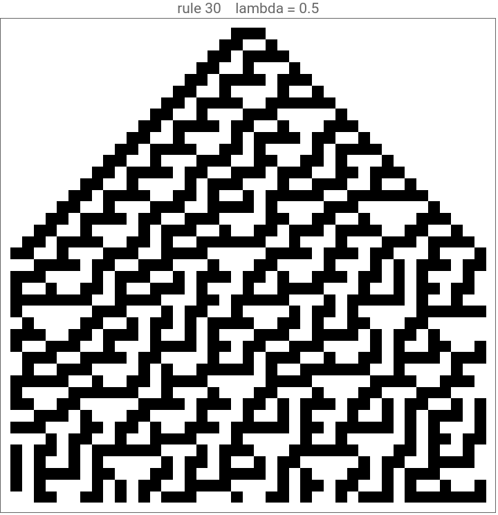
Something above to pay attention to is the quantity lambda, pioneered by computer scientist Christopher Langton to measure the potential for computation in cellular automata. Falling in between 0, which represents pure order, and 1, which represents pure chaos, the most interesting falling in the phase transition between the two. For example, the infamous Rule 30 falls at a lambda of 0.5, which helps indicate random and interesting behavior.
The Market
The Market
Every market tick works as follows, involving every agent within our model. I initialize the model by taking agents and putting them in a row of 21 cells, where the middle three are left black, giving each agent an equal starting state.
Gives three black cells padded on the left and right with nine white cells:
In[]:=
PadRight[{1,1,1},21,0,9]
Out[]=
{0,0,0,0,0,0,0,0,0,1,1,1,0,0,0,0,0,0,0,0,0}
For many of the tests of our model, I run in twenty agent groups. This keeps it under ten percent of the total agents, allowing for independence, while also giving a decent sample size. Below is a visualization of one possible initial state. For this model I only use the two binary states of on/off, and each square has an influence stretching one square.
Generates twenty random agents, and visualizes their initial starting position:
With[{k=2,r=1,nent=20,init=PadRight[{1,1,1},21,0,9]},Column@Table[RandomInteger[{0,k^(k^(2r+1))-1}]->ArrayPlot[{init},MeshTrue],nent]]
Out[]=
12 |
145 |
199 |
151 |
21 |
232 |
235 |
146 |
176 |
211 |
49 |
137 |
192 |
51 |
227 |
182 |
20 |
225 |
94 |
16 |

Next, I partition every agent into random pairs, creating ten potential partners for trade. For a demo, I arbitrarily chose rules 110 and 30, who are three steps into their evolution, and holding three and four cells respectively.
Takes two rules, 110 and 30, and simulates three steps, giving their final number of cells:
In[]:=
demoA=<|"Rule"->110,"State"->Nest[CellularAutomaton[110],PadRight[{1,1,1},21,0,9],3]|>;demoB=<|"Rule"->30,"State"->Nest[CellularAutomaton[30],PadRight[{1,1,1},21,0,9],3]|>;{Total[demoA["State"]],Total[demoB["State"]]}
Out[]=
{3,4}
Potential trade occurs by finding a position where the two strips differ, and then swapping the agents’ values in those regions. The results below documents a position where they differ, and will thus swap position values.
Defines function swapstates, which exchanges agent’s value at a position.
In[]:=
swapstates[{state1_,state2_},posns_List]:={ReplacePart[state1,#->state2[[#]]&/@posns],ReplacePart[state2,#->state1[[#]]&/@posns]}
Finds a cell where two agents differ, and returns the number of that cell, left to right:
In[]:=
demoPos={First@Flatten@Position[demoA["State"]-demoB["State"],1|-1]};{demoV1,demoV2}=swapstates[{demoA["State"],demoB["State"]},demoPos];demoPos
Out[]=
{11}
After trading the value of the strips, each agent “looks” into the future by evolving with its new “production technology,” seeing its potential setup if it evolved after trade.
Looks what would happen after evolving, and returns the number of cells:
In[]:=
demoW1=CellularAutomaton[demoA["Rule"]][demoV1];demoW2=CellularAutomaton[demoB["Rule"]][demoV2];{Total[demoW1],Total[demoW2]}
Out[]=
{6,6}
For comparison purposes, here are the total number of live cells following no trade, and only evolution.
Gives what would happen if they simply advanced another state, with no trading:
In[]:=
demoN1=CellularAutomaton[demoA["Rule"]][demoA["State"]];demoN2=CellularAutomaton[demoB["Rule"]][demoB["State"]];{Total[demoN1],Total[demoN2]}
Out[]=
{5,9}
Generates a table that compares the live cells of two agents, before and after trade/evolution:
In[]:=
s1=demoA["State"];s2=demoB["State"];{t1,t2}={demoV1,demoV2};
In[]:=
Grid[{{"","agent 1 (rule 110)","agent 2 (rule 30)","joint"},{"live cells now",Total[s1],Total[s2],Total[s1]+Total[s2]},{"after one step, no trade",Total[CellularAutomaton[110][s1]],Total[CellularAutomaton[30][s2]],Total[CellularAutomaton[110][s1]]+Total[CellularAutomaton[30][s2]]},{"after one step, with trade",Total[CellularAutomaton[110][t1]],Total[CellularAutomaton[30][t2]],Total[CellularAutomaton[110][t1]]+Total[CellularAutomaton[30][t2]]}},Frame->All]
Out[]=
agent 1 (rule 110) | agent 2 (rule 30) | joint | |
live cells now | 3 | 4 | 7 |
after one step, no trade | 5 | 9 | 14 |
after one step, with trade | 6 | 6 | 12 |
In this example, after a trade and an evolution, the two agents grow from seven alive cells together, to twelve alive cells after. The acceptance test for our trade is based on if the pair’s joint live-cell count rises. If it does, the trade is accepted, and their states are kept. If not, there is no change from their initial state. Even though it would have been more profitable to simply evolve, and not trade, that is not a possibility in this model. Importantly, evolution only happens if the trade is actually accepted. If the trade is not accepted, then each agent remains in its initial state, and does not advance the state of its automata. As our example increased from seven to twelve, the trade is accepted and the evolution goes through.
A function that compares the number of alive cells before and after evolution and trade, dictating whether the model evolves:
In[]:=
moreAliveCellsQ[stateBefore_List,stateAfter_List]:=Total[Flatten[stateBefore]]<Total[Flatten[stateAfter]]
As this process runs, the market additionally stores a series of important information and associations to analyze the data. For example, I track who trades, their rules, the specific swapped positions, the totals before and after, and the final decision. An example of a record looks like the following.
A function which tracks information about our model and the trades within, such as the agents trading and their motivations:
In[]:=
demoRecord=<|"step"->1,"agents"->{1,2},"rules"->{demoA["Rule"],demoB["Rule"]},"positions"->demoPos,"liveBefore"->{Total[demoA["State"]],Total[demoB["State"]]},"liveNoTrade"->{Total[demoN1],Total[demoN2]},"liveAfterTrade"->{Total[demoW1],Total[demoW2]},"accepted"->moreAliveCellsQ[{demoA["State"],demoB["State"]},{demoW1,demoW2}]|>
To expand this to act upon all of the agents, I use the following function. It partitions all of the agents into random pairs, runs the trade-and-evolve stage for each, and records the outcome after the test passes.
An encapsulation of all of the individual parts above:
The above function is combined with the following function runLoggedTF, which threads one stack through T ticks with FoldList, thus returning both the history and the log.
Similar to demoRecord, a function which tracks information and returns the history:
For an example, let’s run the economy for 100 steps.
Initializes agents and runs the economy on a random seed for 100 steps:
Our log tracks one record per attempt, giving us complete data for all successful and attempted trades.
Returns the length of the run:
Graphs data on the steps taken versus the total number of alive cells in the system:
As seen above, total wealth spikes quickly while the rules still have time to grow, before saturating and slowly further increasing. Importantly, in this model wealth will never decrease, as agents will only accept trades if the joint total will increase. However, this does not mean that individual agents will not lose cells, as trades will still be accepted if an agent loses cells, provided that the system as a whole gains a higher joint total. A per-agent picture demonstrating this is below.
Takes each agent and plots their wealth versus time passing:
For another look towards how the economy develops over time, the slider below shows the entire market developing over time. Each row of twenty-one cells is dedicated to one agent, starting with the three alive cells in the middle. Over time, the spikes caused by trade and revolution, as well as the gradual changes can be seen.
Depicts the economy over time, with the trade and evolutions:
Tools for Analysis
Tools for Analysis
As stack recorded every attempt, I need tools to analyze the cellular automata model and try and see if there are any important patterns or trends. First, acceptedRate gives the fraction of attempts that were accepted.
Tracks the percentage of trades accepted:
attribByKey is a tool to credit each attempt to both of its participants, so per-agent and per-rule rates will count correctly. Since every trade involves two agents, finding the acceptance rate per agent requires each attempt to count once for each participant. This put each record into one tagged record for each participant.
Tags each agent involved, counting each participant once:
acceptanceBy groups the acceptance rate by any key, as well as reporting the sample size of the groups to avoid stressing the importance of small groups.
Finds the acceptance rate for any specific agents key, and gives the sample size:
One of the most useful tools is agentLedger, which reveals one agent’s complete trading history, allowing analysis of each agent individually.
Creates a ledger, which reports the trade history of any individual agent:
Mentioned earlier, lambda is a useful measure of complexity which measures the density of a rule, meaning the fraction of its eight cases that output a live cell. Again, automata whose lambda score near 0.5 are the most interesting, with those near 1 and 0 more elementary.
Finds the lambda of each agent, a measure of complexity:
In order to determine how often trade will actually influence the result, I use swapChangesTotal to determine the fraction of attempts where the trade influences the pair’s joint outcome, relative to not trading. This triggers whether it becomes smaller or larger. For example, if the initial state were seven cells, it would trigger at six or eight cells, and not at seven.
Finds the percentage of trades where total cells is affected by the trade:
I also chose to determine the fraction of trades where the swap flipped the acceptance decision itself, denoted by the function decisionFlips.
Finds the percentage of the time that acceptance rate is influenced by the trade:
As seen above , the swap changes the joint outcome in roughly a third of attempts, and ends up flipping the actual decision in a few percent. This compounds greatly, especially over larger runs.
Using acceptanceRate, I can find how often trades are accepted by the market.
Finding the acceptance rate for a mock run:
Additionally, I can see acceptance grouped by the rule densities, or lambdas, of the agent’s rules. In the below example, it can be seen that more complex rules generally have higher acceptance rates, with those around 0.375/0.625 having acceptance rates exceeding 30%. There are outliers to this trend, such as an acceptance rate of 37.5%, which is rather high, for rule number 16, however this is likely explained as more representative of its growth rule.
Finding the acceptance rate of a mock run by lambda score:
I can focus on any agent using agentLedger. Arbitrarily choosing agent 6, I can get the following table. The table documents the agents used, the rules associated with them, and their values before trading, after trading, and with evolution and no trade. Additionally below is a graph documenting the accepts vs. rejects of the associated agent. As might be assumed by agents trading successfully only 24% of the time, agents will often go broads swaths without making trades or evolving the state of their automata.
A ledger, arbitrarily choosing agent 6:
A graph depicting agent 6’s rejects and accepts for trade over time:
Wealth Distribution
Wealth Distribution
Something that was of interest to me was examining the wealth distribution of the model, and seeing if I can determine any trends in the model. I sought to determine if there was inequality in the model, what might be the cause of such inequality, and if there were any noticeable patterns in the distribution of the inequality. To start, I define the function wealthOf, which gives the per-agent wealth of the population.
Finds the wealth of each individual agent in the population:
In order to determine the level of inequality within the system, I chose to use the classic Gini coefficient. Proposed by sociologist Corrado Gini, the Gini coefficient is a common measure of economic inequality, with 0 representing complete economic equality and 1 representing complete inequality. It theoretically could assume scores higher than one given the potential of negative income, however our agents can never seek into debt in our current model. In the modern day, the lowest Gini coefficient is Slovakia, which has a coefficient of around 0.232, with South Africa ranking the highest; after adjustment around 0.52. I introduce the function gini to calculate the coefficient of our model, calculated as the ratio of the area between the line of equality and the Lorenz curve.
Calculates the Gini coefficient of the economy:
Creates a histogram depicting the wealth of individual agents:
Startlingly, the model above models the inequality within the United States very well. The model’s Gini coefficient of 0.421 is only 0.003 from the US’ current rating of 0.418. There is also a clearly identifiable pattern in the histogram, with there being two bi-modal clusters near wealth and poverty, with some agents going straight to 0 and other’s remaining around 18. Given that three agents remained at three throughout the experiment, it is safe to assume that they didn’t make any trades or evolutions throughout the model. There is also a “middle class,” meaning those that end between the poor and the wealthy, but it is small in comparison to either.
To further look through inequality, I used the Lorenz curve, a graphical representation of wealth inequality from American economist Max Lorenz. The graph represents the proportion of overall wealth or income, so for our model’s purposes these are alive cells, which are assumed by the bottom x% of the population. Mentioned above, a completely equal society would have a 45 degree angle from the origin, with the curve below quantifying the level of the inequality. I calculate the inequality using the below function.
Calculates the Lorenz curve of the model:
Plots a graph of the Lorenz curve versus perfect equality in the economy:
The Lorenz curve above “bulges” outward around one-quarter of the way through. In doing so, it indicates that the poor/middle class earn a disproportionately small share of the total resources of the population, an interpretation strengthened by the Gini coefficient from earlier. As seven agents around or below three total cells of wealth will earn less than a single agent that saturates the entirety of the twenty-one cell grid, the rich make proportionally far more than the poor, which explains why they are far closer to the line of equality than the bulge at the bottom.
It is additionally interesting to determine if there are any trends in the development of inequality over time, to see if there are periods where inequality spikes, and where it levels out. Below, the Gini coefficient is calculated at each step.
Calculates the Gini coefficient of the economy over time:
Creates a graph depicting the Gini coefficient versus steps in the economy:
The above model of inequality over time depicts how it starts at perfect equality, with everyone owning the same three alive cells, before immediately correcting to a Gini coefficient of 0.320 by step 2. As time continues, it continues to spike, with large jumps occurring from 0.320 to 0.418, and 0.419 to 0.466 taking place over a single turn. However, after reaching a peak around step 25, inequality steadily decreased over time, reaching the point that accurately modeled the United States. This phenomenon is likely explained by the fact that agent’s wealth is largely obtained within the first few trades, as it is at that point where they can grow the most. Following those periods of immense growth, trade becomes an increasingly important phenomenon for the poor cells, as it can give them an arrangement that allows them to escape their current pattern, and thus can slightly level out the spikes of inequality.
An additionally interesting point of consideration is the complexity, or lambda, of the rule, plotted versus the final wealth of each agent. It can be conjectured that more complex agents, with thusly higher lambdas, will be more successful than less complex agents. Below is a graph that plots the final wealth versus the rule density of each agent:
Creates a graph plotting final wealth versus rule density:
Seen above, there is a moderately strong positive correlation between final wealth and the rule density of each agent. Though certainly not linear, and with clear outliers such as one agent having 17 cells and a lambda of 0.25, there is certainly an upward trend. This supports the idea that complexity is generally useful in trade.
In order to fully determine these trends, I ran the model economy in 200 independent economies, so that it can be ensured that these trends were not outliers. The below function runs our economy 200 times.
Creates a series of random agents and economies, running tests again:
Below is the visualization of our results:
Creates a histogram of the results of the model economies:
The above visualization confirms the trend of the histogram from earlier. There is a large split between the wealthy and the poor who dominate the graph, with a depression in the middle of the graph demonstrating how the middle class is very small in this model. Most interestingly, there is a large portion of agents who remain stuck as three cells, as they are never motivated to trade if their cell will quickly lose cells. This may mirror the general idea of an autarky. These trends are largely explained by the fact that the growth of cells is determined by their production capabilities, or cells, so an agent’s fortune tracks its future movement. Generally, this bi-modal graph mimics other classic kinetic-exchange models from economics, and indicates cellular automata as a viable modeling method.
Rule Class
Rule Class
Another interesting thing to examine, which naturally comes hand-in-hand with cellular automata, is the rule class of each agent. Classified by Wolfram, there are four general classes, where 1 is associated with uniform, 2 is associated with periodic, 3 is associated with chaotic rules, and 4 is associated with complex rules. Classes 1 through 2 are empirically determined from each rule’s dynamics, seen by evolving it from a random start and then perturbing one cell. If the pattern collapses to a uniform state, it is class 1; if the perturbation stays bounded, it is class 2; if it spreads across the lattice, class 3. Class 4 are the well-established complex rules, which are categorized for their unique behavior. Given that classification of elementary rules is at time subjective, the boundary between classes 2 and 3 is partially fuzzy.
First, let’s visualize the rules that collapse to a uniform state.
Lists the Class 1 rules and shows their visualization after thirty moves:
Now, rules that are deemed chaotic.
Lists the class three rules and depicts them after thirty moves:
Finally, the following 6 rules are acknowledged as complex.
Lists the class four rules and depicts them after thirty generations:
All of the other rules immediately default to class 2.
Labels all other unnamed rules to class 2:
In order to determine trends among rules, I can pool the final wealth over 150 runs, with final results grouped by each agent’s rule class.
Creates a random seed of agents and their wealth, and groups the rules by their class:
The following chart summarizes the results of the runs by class. It gives the total number of agents from each class, the mean of each agent among the class, as well as the median of the agents.
Depicts the rule classes in a table, and the mean and median of their average live cell count:
To visualize the results, it can be put into a box-whisker chart:
Depicts the above data in a box-whisker chart:
It is important to note that despite class 1 having the highest 75th percentile, this is largely driven by outliers. They have by far the smallest median, with it landing at only around four cells. Their mean of 9.18 is therefore also likely skewed heavily upwards, with over 25% of agents landing twenty-one cells, and heavily skewing the rest of the population. The most generally successful rule class can thus be seen as class three, which are determined as the most chaotic functions, as they have both the highest mean and median among the rule-classes. It is also important to note how class two agents make up by far the majority of the agents in the economy, with 2,159 agents out of the 3,000 total during these simulations.
Given that the majority of the agents were class 2, I sought to answer whether rule classes shaped who trades with whom. For example, if class 2 agents were especially adverse to trading with class 1 agents, that might explain their general struggles, as it would leave around 70% of the population unviable trade partners. Learning what pairs of classes tend to trade, and thus have room to grow together, could indicate the “role” of specific classes of agents in the mock economy.
Starting the analysis, I can pool the trade logs of the recent runs.
Creates a random seed, and pools the trade logs of the runs:
Using the tool acceptanceBy from earlier, I can determine the acceptance rate by class pair.
Determines the acceptance rate between two different classes, and depicts in chart:
For easier analysis, I can render this as a class-by-class heat map, which gives us some trends.
Visualizes data as a heat map:
The above heat map reveals some interesting trends amongst the rule classes. Perhaps most prominently, two agents that are both class 4 trade by far the most often between any specific class, with their rate of 0.5 exceeding the typical baseline of 0.24 by more than double. Additionally of note is that agents of rule class 1 are more likely to trade than any other class. From the table, they had trade acceptance rates of 0.34, 0.31, 0.23, and 0.27 with rule classes 1, 2, 3, and 4 respectively. Besides their trade rates with 0.23, which was narrowly below the baseline, their trade levels exceeded all of the others. In contrast, the class which traded the least was class 3, with only 0.19 of trades clearing between two class 3 agents.
These trends are especially interesting when considering how rule class generally corresponded to final wealth. The one’s that traded the most, class 1, generally ended up the poorest, while those that traded the least, class 3, generally ended up the richest.
I also thought it would be fruitful to determine what level of success each of the individual 256 rules reach, in order to see which programs in particular make progress, and therefore glean possible patterns. To do this, for each of the 256 rules, I place one agent with that rule in a population of 19 random partners, run the market, and average each agent’s final wealth across all the runs to see their general fitness. I define a function popWithTarget, a population with a chosen target rule.
Creates a population with one target rule and nineteen other random agents:
In order to find the mean final wealth of the target, I define a function fitnessOf.
Finds the fitness of an agent across several runs:
And, to run all 256 rules, I run a sweep and end up with 5120 runs in total.
Runs each rule twenty times, giving a dataset for each agent’s average outcome:
Visualizing this, I can create the following table, colored by the rule classes from above.
Depicts the above data in a chart, categorized by class:
The landscape above is quite interesting, with a few clearly discernible patterns, such as periodically repeating groups clustered between 3-8 and 15-20 cells, both repeating around every thirty rules. Class 2 is quite divisive, with most rules falling between 15-20 or 3-8, and not many “middle class” rules. In fact, there is a large lack of “middle class” rules in general, with the few dots sparsely populating the middle region being class 1 cells. Class 1 cells form an equally divisive group, either saturating their cells or completely vanishing most of the time. Class 3 cells on average were generally closer than most of the other classes, and from earlier often the richest, at the cost of having lower peaks. They generally clustered between 6-10 and 15-18.
Mobility
Mobility
Another topic of interest was determining the mobility available in the market, or if the cellular automata which were poor could recover wealth. Trade would hopefully prevent fortunes “locking in,” as it provides an avenue to get a cell turned alive, and thus influence it’s neighbor cells. To do this, I first define the function wealthMat, which determines the per-agent wealth at each step of the process running.
Determines each agents wealth at each step of the process:
In order to determine the mobility in the economy, I chose to compare the result that wealth at different steps had with the final wealth of individual agents. To understand the magnitude of the relationship, I used Spearman’s correlation coefficient, a function pioneered by American psychologist Charles Spearman, which compares two variables that are monotonically related. It is defined as the Pearson correlation coefficient between the rank values. In order to calculate the value, I define the following function lockIn.
Determines and visualizes the Spearman correlation coefficient between final ranking and ranking at various steps:
The above graph demonstrates that the wealth of agents early into the market is largely reflective of their final wealth. Even only eight steps from the initial state, the Spearman correlation coefficient exceeds 0.5, indicating moderate strength in the relationship. By the fourteenth step, it reaches past 0.8, and other than small changes induced by change, one’s wealth is largely determined. This makes sense in the context of the model, given that one’s live cell count is responsive to its production (automata rule), and trade can only change one cell each cycle.
Another way of understanding how long wealth persists is through comparing average rank correlation at increasing time lags. This simply means taking the initial value at a point, and looking 5, 10, 15 steps in the future, and comparing that to the initial value, with the proportion giving how long wealth can typically be expected to last. To do so, I define and use the function lagAuto.
Determines how long on average it takes to shift from one’s wealth ranking:
As can be seen above, the wealth ranking is very persistent, even as it steadily decreases. Despite thirty steps being made, the wealth ranking remains with a coefficient near 0.85, indicating a very strong relationship between the initial and later states. This is further evidence that trade in this model is not radically distributive, and instead institutes small changes which can at times have a large impact on the fortunes of an individual agent. Most of the time however, the productivity of an agent is mainly determined by the productivity of its automata rule and individual state, and fortunes lock in rather quickly.
Baselines
Baselines
In order to better understand the model, it is important to isolate the contribution of trade by running a few baselines, and see what the effect of trade versus a vacuum is. For baselines, I ran a no-trade baseline, which describes the same general transact function, with the same pair selection, same evolution, etc., but refuses to ever swap cells. As such, the difference from the model is the contribution of exchange.
Runs the transact function without trading:
And, to accompany it, the matching logging function.
Logs the trade function without exchange:
The other baseline ran in this section is the random-accept baseline, where I keep the swap, but replace the acceptance test, which needs an increase in joint utility, to a 0.5 chance. This makes it so that the difference is the contribution of the screening for a necessity of growth, and can help determine if “intelligent” trades create any sort of difference. To do so, I use the function randomAcceptQ, which ignores the argument of moreAliveCellsQ.
Runs the transact function, randomly accepting trades 50% of the time:
For both of these baselines, I generate another random population, using the same construction I normally use in this essay with twenty agents.
Generates another random population with twenty agents:
Next, I ran 200 economies per condition from the same random seed.
Runs 200 economies from random seeds for each baseline, creating possible comparisons:
For these baselines, I chose to calculate the following summary statistics. I chose to calculate mean wealth of cells, the mean of the Gini coefficient each run, the fraction of agents that reach zero cells, and the fraction of agents that saturate and reach twenty-one cells.
Calculates the inequality, wealth, and percentage of agents who reach 0 or 21:
Depicts the above data in a table:
Visualizes the data in a histogram:
The above data indicates that the filter part of the trade function, where they refuse trades which are harmful, is largely the most important. The agents that randomly-accept cost around 2 cells per agent, with it falling far behind both the normal model and the no-trade baseline once total wealth is summed. Additionally, randomly accepting leads to higher inequality, with the mean Gini coefficient exceeding the other baselines by several percentage points. This can be especially seen in the far larger percentage of agents which hit zero in the random-accept baseline, which is likely explainable by how they get taken advantage of without the utility filter. In comparing the trade model with the no-trade model, it can be seen that trade has a definite advantage over regular evolution. Under trade, there is both less inequality, around 2%, and around 0.2 more live cells per agent. Over 500 seeds, it evidences that trade almost always has an advantage over autarky in inequality and wealth.
Trade Balance
Trade Balance
Another natural question to ask of any economy is the direction of trade. I wanted to determine which agents tended to be net exporters, giving away more cells than they take, and which tended to be net importers, meaning they take more cells than they gave. Economic theory has often been contentious on this fact; for example, the mercantilist theory that dominated medieval Europe proposed that a nation grows rich by exporting more than it imports and hoarding the bullion difference. Using the log records from earlier, I can test this, as it records what each agent gives and takes in accepted swaps. Below, I define a fuction tradeBalance, which computes each agent’s net cells imported across a run and places it against final wealth.
Determines and plots the relationship between exported and imported cells versus the final wealth of individual agents:
Interestingly, in the preliminary run, there is a clearly negative relationship between the net exports and the final wealth of individual agents. Admittedly, there is very large variance, such as plenty of successful agents with either zero or one cells imported. However, the agents that have exported more than -4 cells are wildly successful, while those that have imported two or more are far less opportune. In order to confirm these trends, it is logical to run these tests again, with a larger sample set. The following, as usual, pools two hundred independent runs and measures the correlation between imports and final wealth again.
With a random population, determines the correlation coefficient over a sizable dataset:
From running several tests, it can be seen that there is a slight negative correlation between imports and final wealth, with countries that export more generally being more successful. This can be seen as a result of their production technology (rule), being vastly more powerful than general agents. Those that saturate, or nearly saturate, the grid will have far more cells that they can trade, and will likely fill it after a trade, meaning they can accept and export a large percentage of the trades. In this lens, it can be seen as generally in line with mercantilist thought, which prioritizes having a strong industrial base, here a rule, and further developing for exporting more wealth.
As a final portion of analysis, I examined the differences between the richest and poorest agents directly, averaging their trade balance to do so.
Determines the typical trade balance of the richest and poorest agents in the model:
Confirming the above negative trend, it can be seen that there is roughly a half a cell difference between cells imported and exported from rich and poor agents. Additionally, this indicates that nearly all poor agents ended up being net importers, a conclusion which may cast worry upon over-reliance on external countries.
Future Directions
Future Directions
Looking forward, I would like to see if I could expand the model, and use it to model real-world events and economic phenomena. There are other types of utility preferences other than number of alive cells that I would like to explore in the future, and I would be interested in seeing if a heterogenous preferences or Pareto efficient model would be possible to make. Additionally, I would like to model economic catastrophes, such as supply shocks, inflation, and more in this model, and see if it reflects similar patterns to what I see in the real world, and why. Beyond just exploring real-world events and phenomena, I believe it would be productive to expand this project by manipulating some of the assumptions of the model, such as that there is a binary between alive and dead cells, and that only one cell is traded at a time.
Conclusion
Conclusion
This project focused upon taking the incredibly complex idea of economic trade and its associated phenomena, and sought to analyze it through the medium of cellular automata. By modeling trade in this way, and seeing if the familiar features of a trading economy would emerge, I sought to determine if a simplistic yet effective model could be made. Starting from identical, isolated endowments of three cells, several of the regular aspects of a real-world model were generated by the minimal computational economy. Inequality, measured at a degree which closely mimics that of our modern world nations, emerges from the equal start. Wealth generally comes as a result of an agent’s productive capacity, or rule, rather than a medium of exchange. Final results are often predicated upon early divergences, with a few places where trade can undo initial placement. Trade itself brings an edge over autarky with both inequality and wealth, and the richest agents turn out to be net exporters of cells. Overall, the project demonstrates how much of economic structure appears from agents that are nothing more than small programs trading single cells.
Acknowledgments
Acknowledgments
Most importantly, I would like to thank my mentor Daniel Sanchez for supporting me throughout this project, keeping me on track, helping me organize and implement my ideas, and setting up meetings for me in order to better understand my project and my goals. This project would not have been possible without their guidance and support, and their dedication shaped not only the final product, but the passion and work behind it. I am forever grateful for having the opportunity to work with them.
I would also like to thank the TA’s in this program for their insight, encouragement, and commitment towards making this program worthwhile. Their expertise and experience with math and coding helped meld the project into what it ultimately became. I would also like to thank the program directors, Rory Foulger, Megan Davis, and Eryn Gillam for giving me the opportunity to be part of this program. Finally, I would like to thank Dr. Stephen Wolfram for suggesting this project, a decidedly unique approach to economic trade.
I would also like to thank the TA’s in this program for their insight, encouragement, and commitment towards making this program worthwhile. Their expertise and experience with math and coding helped meld the project into what it ultimately became. I would also like to thank the program directors, Rory Foulger, Megan Davis, and Eryn Gillam for giving me the opportunity to be part of this program. Finally, I would like to thank Dr. Stephen Wolfram for suggesting this project, a decidedly unique approach to economic trade.
References
References
◼
Four Classes of Behavior: A New Kind of Science | Online by Stephen Wolfram [Page 231]. (n.d.). www.Wolframscience.Com. Retrieved July 2, 2026, from https://www.wolframscience.com/nks/p231--four-classes-of-behavior/
◼
Seifter, J., & Reggia, J. A. (2015). Lambda and the Edge of Chaos in Recurrent Neural Networks. Artificial Life, 21(1), 55–71. https://direct.mit.edu/artl/article-abstract/21/1/55/2790/lambda-and-the-edge-of-chaos-in-recurrent-neural?redirectedfrom=fulltext
◼
World Population Review. (2025). Gini Coefficient by Country 2025. World Population Review. https://worldpopulationreview.com/country-rankings/gini-coefficient-by-country
CITE THIS NOTEBOOK
CITE THIS NOTEBOOK
A model of economic trade using cellular automata
by Lucas Fugate
Wolfram Community, STAFF PICKS, July 9, 2026
https://community.wolfram.com/groups/-/m/t/3749738
by Lucas Fugate
Wolfram Community, STAFF PICKS, July 9, 2026
https://community.wolfram.com/groups/-/m/t/3749738